How-to: Convert a timml model to timflow

Conversion of a timml model to a timflow model only requires a few minor changes.

The import statement

The timflow.steady model is essentially the same as timml. So all that is required is to change the import statement. For example, if your model imports timml as

import timml

and you don’t want to make any other changes to your model, then replace the import statement by

from timflow import steady as timml

or, if you like that better

import timflow.steady as timml

If you used a different name in your original model, then make sure to use the same name in the timflow model. So if your import statement was

import timml as tml

then replace it by

import timflow.steady as tml

Note: The docs of timflow use the three-letter abbreviation tfs (for timflow steady) for the steady model.

Combining two or more plot statements on the same graph

All plotting commands in timflow are gathered in the plots submodule. Each plotting command optionally takes an axis as input. If no axis is provided, then a new plot is created. Each plotting command returns the axis to which is plots. When you issue multiple plotting commands in a row, for example to first plot contours and then on the same graph plot tracelines, then make sure that the axis created by the contouring command is passed to the tracelines command. For example, consider the following model of a well in uniform flow

import timflow.steady as tfs

ml = tfs.ModelMaq(kaq=10, z=[10, 0])
rf = tfs.Constant(ml, xr=-1000, yr=0, hr=41)
uf = tfs.Uflow(ml, slope=0.001, angle=0)
w = tfs.Well(ml, xw=-400, yw=0, Qw=50.0, rw=0.2)
ml.solve()

Number of elements, Number of equations: 3 , 1
.
.
.

solution complete

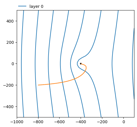
A contour plot is created and the returned axis is stored in the variable ax0. Then a traceline is computed and added to the same graph by supplying the ax=ax0 as input.

ax0 = ml.plots.contour(win=[-1000, 100, -500, 500], ngr=50, levels=10, labels=False)
ml.plots.tracelines(
    xstart=[-800], ystart=[-200], zstart=[1], hstepmax=20, color="C1", ax=ax0
)

.

[<Axes: >]

Note that two separate graphs are created when the ax=ax0 input is omitted. You won’t even see much on the second graph, as no window is provided (like the win=[-1000, 100, -500, 500] specification for the contours). The window is set by default to a very large area if no ax is provided and no win.

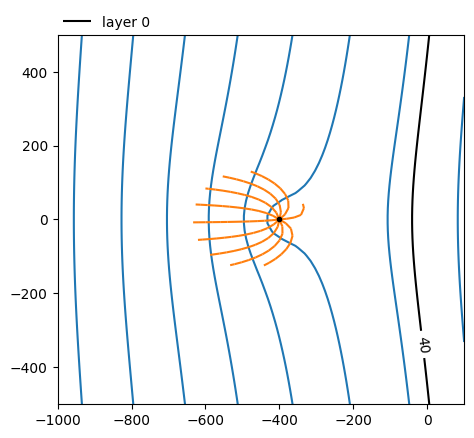
The same procedure holds for combining other plots. For example combining two contour plots, or a contour plot plus a capture zone. Note that the plotcapzone function has moved to the plots module. All three can be combined as follows

ax0 = ml.plots.contour(win=[-1000, 100, -500, 500], ngr=50, levels=10, labels=False)
ml.plots.plotcapzone(
    well=w, nt=10, zstart=[1], hstepmax=20, tmax=10 * 365, color="C1", ax=ax0
)
ml.plots.contour(win=[-1000, 100, -500, 500], ngr=50, levels=[40], color="k", ax=ax0);

.
.
.
.
.
.
.
.
.
.

Renaming of elements

If you had not updated your timml model recently, you may not have noticed that some old element names have been replaced by newer more descriptive ones. This was done in version 6.8.0. The old ones still work, but you will get a deprecation warning. These are the changes:

Line-sinks

• HeadLineSink -> River

• HeadLineSinkString -> RiverString

• LineSinkDitch -> Ditch

• LineSinkDitchString -> DitchString

Line-doublets

• ImpLineDoublet -> ImpermeableWall

• ImpLineDoubletString -> ImpermeableWallString

• LeakyLineDoublet -> LeakyWall

• LeakyLineDoubletString -> LeakyWallString

Xsection elements

• HeadLineSink1D -> River1D

• ImpLineDoublet1D -> ImpermeableWall1D

• LeakyLineDoublet1D -> LeakyWall1D

New elements

In timml release 6.8.0 and before, a bunch of new elements were introduced that may be worth checking out:

• WellString: A string of wells for which the total discharge is given. The discharge is distributed over the wells such that the head inside the wells is the same for all wells. This element is intended for wells connected by a manifold and a single pump.

• TargetHeadWell: A well for which a target head is specified at a target location. The discharge is computed to meet the specified head at the target location.

• TargetHeadWellString: Like a string of wells, but now the total dicharge is computed such that the specified head is met at the the target location.

• RadialCollectorWell: A radial collector well with an arbitrary number of arms. The total discharge of the radial collector well is specified and is distributed across the arms such that the head is uniform and equal along all arms.

• BuildingPitMaq: A special inhomogeneity element to simulate sheet piles around a building pit. For use in a ModelMaq model.

• BuildingPit3D: A special inhomogeneity element to simulate sheet piles around a building pit. For use in a Model3D model.