Connected Wells#
WellString elements can be used to model a series of connected wells. There are several types of WellString:
WellString: connected wells with equal head inside the wells and a user-specified total dischargeHeadWellString: connected wells with equal specified head inside the wells, this is identical to specifying multiple HeadWells.TargetHeadWellString: connected wells with equal head inside the wells and one user-specified head at a point \((x_c, y_c)\)
This notebook shows how to model the WellString and TargetHeadWellString elements
and compares the results to models with individual wells. Examples are shown for both
elements in single- and multi-layer models.
import matplotlib.pyplot as plt
import numpy as np

import timflow.steady as tfs
WellString#
A series of wells that have equal head (pressure) inside the well and pump with a total specified discharge.
Single-layer model#
# model parameters
kh = 10  # m/day

ctop = 1000.0  # resistance top leaky layer in days

ztop = 0.0  # surface elevation
zbot = -20.0  # bottom elevation of the model

z = [1.0, ztop, zbot]
kaq = np.array([kh])
c = np.array([ctop])
Reference model with 2 wells with equal discharge
mlref0 = tfs.ModelMaq(kaq=kaq, c=c, z=z, topboundary="semi", hstar=0)
w1 = tfs.Well(mlref0, 0, -10, Qw=50, rw=0.1)
w2 = tfs.Well(mlref0, 0, 10, Qw=50, rw=0.1)
mlref0.solve()
Number of elements, Number of equations: 3 , 0
No unknowns. Solution complete
Reference model with 2 head-specified wells, specifying the head inside well w1 computed with the previous model.
mlref1 = tfs.ModelMaq(kaq=kaq, c=c, z=z, topboundary="semi", hstar=0)
wh1 = tfs.HeadWell(mlref1, 0, -10, hw=w1.headinside().item(), rw=0.1)
wh2 = tfs.HeadWell(mlref1, 0, 10, hw=w1.headinside().item(), rw=0.1)
mlref1.solve()
Number of elements, Number of equations: 3 , 2
.
.
.

solution complete
Model with a WellString that has total discharge equal to the sum of the two discharge-specified wells.
ml0 = tfs.ModelMaq(kaq=kaq, c=c, z=z, topboundary="semi", hstar=0)
ws = tfs.WellString(ml0, xy=[(0, -10), (0, 10)], Qw=100, rw=0.1)
ml0.solve()
Number of elements, Number of equations: 2 , 2
.
.

solution complete
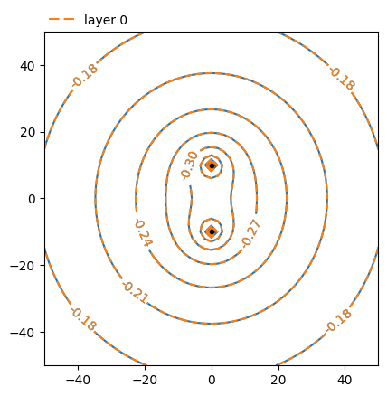
Contour the heads of the first reference model and the WellString model.
levels = 10
ax = mlref0.plots.topview(win=(-50, 50, -50, 50))
mlref0.plots.contour(
    win=(-50, 50, -50, 50),
    ngr=51,
    levels=levels,
    decimals=2,
    layers=[0],
    ax=ax,
)
ml0.plots.contour(
    win=(-50, 50, -50, 50),
    ngr=51,
    levels=levels,
    decimals=2,
    layers=[0],
    linestyles="dashed",
    color="C1",
    ax=ax,
);
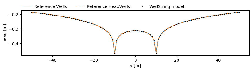
Compare heads along y between all 3 models (2 reference models and the WellString model).
y = np.linspace(-50, 50, 101)
x = np.zeros_like(y)
href = mlref0.headalongline(x, y)
href2 = mlref1.headalongline(x, y)
h0 = ml0.headalongline(x, y)

plt.figure(figsize=(10, 2))
plt.plot(y, href[0], label="Reference Wells")
plt.plot(y, href2[0], "--", label="Reference HeadWells")
plt.plot(y, h0[0], "k.", ms=3, label="WellString model")
plt.xlabel("y [m]")
plt.ylabel("head [m]")
plt.legend(loc=(0, 1), frameon=False, ncol=3);
Check computed discharges
# 2 discharge wells, Q specified not computed
w1.discharge(), w2.discharge()
(array([50.]), array([50.]))
# 2 HeadWells
wh1.discharge(), wh2.discharge()
(array([50.]), array([50.]))
# WellString
ws.discharge_per_well()
array([[50., 50.]])
Compare heads inside the wells
# 2 discharge wells
w1.headinside(), w2.headinside()
(array([-0.46739383]), array([-0.46739383]))
# 2 HeadWells, specified, not computed
wh1.headinside(), wh2.headinside()
(array([-0.46739383]), array([-0.46739383]))
# WellString
ws.headinside(), ws.wlist[0].headinside(), ws.wlist[1].headinside()
(np.float64(-0.4673938257716392), array([-0.46739383]), array([-0.46739383]))
Multilayer model#
The following example compares the WellString element to reference models with individual Wells and HeadWells in an aquifersystem consisting of 3 layers. In this example, all wells are screened in the bottom two aquifers.
# model parameters
kh = [5, 10, 20]  # m/day

c = [1000.0, 100.0, 1.0]  # resistance leaky layers in days

ztop = 0.0  # surface elevation
zbot = -50.0  # bottom elevation of the model

z = [1.0, ztop, -10, -15, -25, -26, zbot]
kaq = np.array(kh)
c = np.array(c)
Reference model with discharge wells
mlref2 = tfs.ModelMaq(kaq=kaq, c=c, z=z, topboundary="semi", hstar=0)
w1 = tfs.Well(mlref2, 0, -10, Qw=50, rw=0.1, layers=[1, 2])
w2 = tfs.Well(mlref2, 0, 10, Qw=50, rw=0.1, layers=[1, 2])
mlref2.solve()
Number of elements, Number of equations: 3 , 4
.
.
.

solution complete
Reference model with head-specified wells
mlref3 = tfs.ModelMaq(kaq=kaq, c=c, z=z, topboundary="semi", hstar=0)
wh1 = tfs.HeadWell(mlref3, 0, -10, hw=w1.headinside(), rw=0.1, layers=[1, 2])
wh2 = tfs.HeadWell(mlref3, 0, 10, hw=w1.headinside(), rw=0.1, layers=[1, 2])
mlref3.solve()
Number of elements, Number of equations: 3 , 4
.
.
.

solution complete
Model with WellString
ml1 = tfs.ModelMaq(kaq=kaq, c=c, z=z, topboundary="semi", hstar=0)
ws = tfs.WellString(ml1, xy=[(0, -10), (0, 10)], Qw=100, rw=0.1, layers=[1, 2])
ml1.solve()
Number of elements, Number of equations: 2 , 4
.
.

solution complete
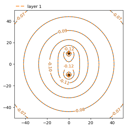
Compare head contours
ilay = 1
levels = 10
ax = mlref2.plots.topview(win=(-50, 50, -50, 50))
mlref2.plots.contour(
    win=(-50, 50, -50, 50),
    ngr=51,
    levels=levels,
    decimals=2,
    layers=[ilay],
    ax=ax,
)
ml1.plots.contour(
    win=(-50, 50, -50, 50),
    ngr=51,
    levels=levels,
    decimals=2,
    layers=[ilay],
    linestyles="dashed",
    color="C1",
    ax=ax,
);
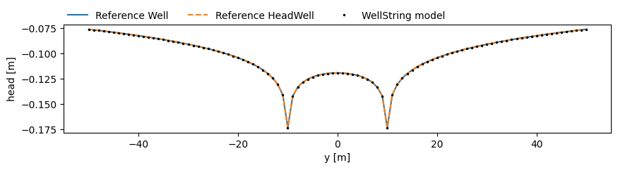
Compare drawdowns along y
y = np.linspace(-50, 50, 101)
x = np.zeros_like(y)
href2 = mlref2.headalongline(x, y)
href3 = mlref3.headalongline(x, y)
h1 = ml1.headalongline(x, y)

ilay = 1
plt.figure(figsize=(10, 2))
plt.plot(y, href2[ilay], label="Reference Well")
plt.plot(y, href3[ilay], "--", label="Reference HeadWell")
plt.plot(y, h1[ilay], "k.", ms=3, label="WellString model")
plt.xlabel("y [m]")
plt.ylabel("head [m]")
plt.legend(loc=(0, 1), frameon=False, ncol=3);
Compare discharges
# 2 discharge wells, total Q specified
w1.discharge(), w2.discharge()
(array([ 0.        ,  8.66671446, 41.33328554]),
 array([ 0.        ,  8.66671446, 41.33328554]))
# 2 head specified wells
wh1.discharge(), wh2.discharge()
(array([ 0.        ,  8.66671446, 41.33328554]),
 array([ 0.        ,  8.66671446, 41.33328554]))
# WellString, transposed to compare to above
ws.discharge_per_well().T
array([[ 0.        ,  8.66671446, 41.33328554],
       [ 0.        ,  8.66671446, 41.33328554]])
Compare heads
# 2 discharge wells
w1.headinside(), w2.headinside()
(array([-0.17338765, -0.17338765]), array([-0.17338765, -0.17338765]))
# 2 HeadWells, specified, not computed
wh1.headinside(), wh2.headinside()
(array([-0.17338765, -0.17338765]), array([-0.17338765, -0.17338765]))
ws.headinside(), ws.wlist[0].headinside(), ws.wlist[1].headinside()
(np.float64(-0.17338765212543442),
 array([-0.17338765, -0.17338765]),
 array([-0.17338765, -0.17338765]))
TargetHeadWellString#
A series of connected wells with equal head (pressure) inside all wells and a specified
head at one point \((x_c, y_c)\) and layer. By default the specified head is applied in layer
0, but this can be set with lcp=<layer>in the TargetHeadWellString element.
Single layer example#
# model parameters
kh = 10  # m/day

ctop = 1000.0  # resistance top leaky layer in days

ztop = 0.0  # surface elevation
zbot = -20.0  # bottom elevation of the model

z = [1.0, ztop, zbot]
kaq = np.array([kh])
c = np.array([ctop])

# point at which head is specified
xcp = 10.0
ycp = 0.0
hcp = -2.0  # specified head at (xc, yc)
Create a model with a TargetHeadWellString.
ml2 = tfs.ModelMaq(kaq=kaq, c=c, z=z, topboundary="semi", hstar=0)
ws = tfs.TargetHeadWellString(ml2, [(0, -10), (0, 10)], rw=0.1, hcp=hcp, xcp=10, ycp=0)
ml2.solve()
Number of elements, Number of equations: 2 , 2
.
.

solution complete
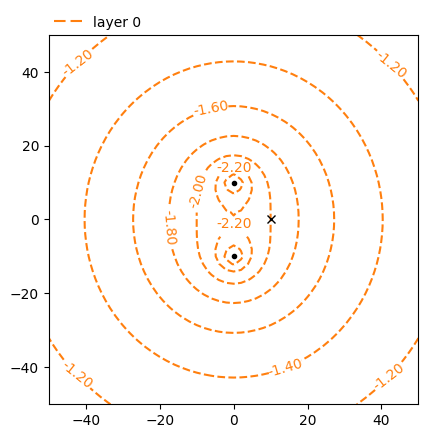
Plot the head contours for the model and mark location of the head target.
ilay = 0
levels = [-2.4, -2.2, -2.0, -1.8, -1.6, -1.4, -1.2]
ml2.plots.contour(
    win=(-50, 50, -50, 50),
    ngr=51,
    levels=levels,
    decimals=2,
    layers=[ilay],
    newfig=False,
    linestyles="dashed",
    color="C1",
)
plt.plot(ws.xcp, ws.ycp, "kx");
/home/docs/checkouts/readthedocs.org/user_builds/timflow/envs/27/lib/python3.13/site-packages/timflow/steady/plots.py:119: UserWarning: The following kwargs were not used by contour: 'newfig'
  cs = ax.contour(xg, yg, h[i], levels, colors=c[i], **kwargs)
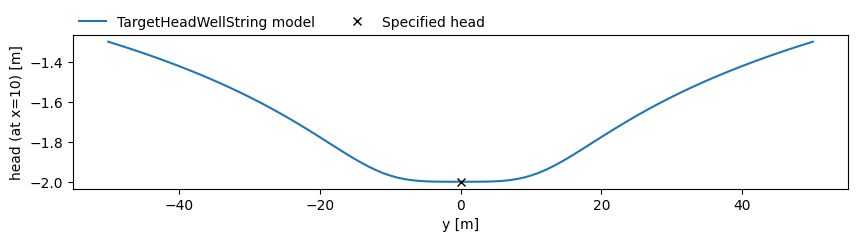
Plot the head along y at x=10, to show that the specified head is met
y = np.linspace(-50, 50, 101)
x = ws.xcp * np.ones_like(y)
h2 = ml2.headalongline(x, y)

ilay = 0
plt.figure(figsize=(10, 2))
plt.plot(y, h2[ilay], label="TargetHeadWellString model")
plt.plot(ws.ycp, ws.hcp, "kx", label="Specified head")
plt.ylabel("head (at x=10) [m]")
plt.xlabel("y [m]")
plt.legend(loc=(0, 1), frameon=False, ncol=3);
Compute the discharge per well
# TargetHeadWellString model, shape: (nlay, nwells)
ws.discharge_per_well()
array([[351.90536633, 351.90536633]])
Compare heads inside the well
# TargetHeadWellString
ws.headinside(), ws.wlist[0].headinside(), ws.wlist[1].headinside()
(np.float64(-3.2895679095614803), array([-3.28956791]), array([-3.28956791]))
Multi-layer example#
An example of a TargetHeadWellString in a multi-layer model.
# model parameters
kh = [5, 10, 20]  # m/day

c = [1000.0, 100.0, 1.0]  # resistance leaky layers in days

ztop = 0.0  # surface elevation
zbot = -50.0  # bottom elevation of the model

z = [1.0, ztop, -10, -15, -25, -26, zbot]
kaq = np.array(kh)
c = np.array(c)

# point at which head is specified
xcp = 10.0
ycp = 0.0
hcp = -2.0  # specified head at (xc, yc)
lcp = 1  # layer
Create a model with a TargetHeadWellString.
ml3 = tfs.ModelMaq(kaq=kaq, c=c, z=z, topboundary="semi", hstar=0)
ws = tfs.TargetHeadWellString(
    ml3,
    xy=[(0, -10), (0, 10)],
    rw=0.1,
    layers=[0, 1, 2],
    hcp=hcp,
    xcp=xcp,
    ycp=ycp,
    lcp=lcp,
)
ml3.solve()
Number of elements, Number of equations: 2 , 6
.
.

solution complete
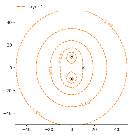
Plot the head contours in the reference model and the TargetHeadWellString model.
ilay = 1
levels = [-2.4, -2.2, -2.0, -1.8, -1.6, -1.4, -1.2]
ml3.plots.contour(
    win=(-50, 50, -50, 50),
    ngr=51,
    levels=levels,
    decimals=2,
    layers=[ilay],
    newfig=False,
    linestyles="dashed",
    color="C1",
)
plt.plot(ws.xcp, ws.ycp, "kx");
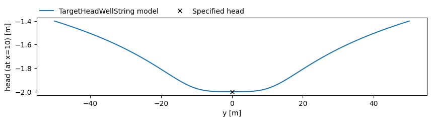
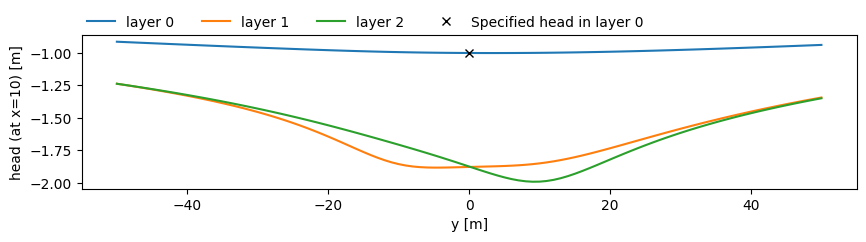
Plot the head along y=10 to show that the head target is met.
y = np.linspace(-50, 50, 101)
x = ws.xcp * np.ones_like(y)
h3 = ml3.headalongline(x, y)

ilay = lcp
plt.figure(figsize=(10, 2))
plt.plot(y, h3[ilay], label="TargetHeadWellString model")
plt.plot(ws.ycp, ws.hcp, "kx", label="Specified head")
plt.ylabel("head (at x=10) [m]")
plt.xlabel("y [m]")
plt.legend(loc=(0, 1), frameon=False, ncol=3);
Compare discharges
# TargetHeadWellString, discharge, shape : (nlay, nwells)
ws.discharge_per_well()
array([[ 78.6860849 ,  78.6860849 ],
       [149.29528764, 149.29528764],
       [716.30768959, 716.30768959]])
Compare heads inside the well
# TargetHeadWellString
ws.wlist[0].headinside(), ws.wlist[1].headinside()
(array([-3.09424294, -3.09424294, -3.09424294]),
 array([-3.09424294, -3.09424294, -3.09424294]))
Compute head at specified point
# TargetHeadWellString
ml3.head(xcp, ycp)
array([-1.94106669, -2. , -2.00047328])
Different layers per well#
The WellString elements allow the specification of different layers per well, as shown in the example below.
ml4 = tfs.ModelMaq(kaq=kaq, c=c, z=z, topboundary="semi", hstar=0)
ws = tfs.TargetHeadWellString(
    ml4, xy=[(0, -10), (0, 10)], rw=0.1, layers=[(1,), (2,)], hcp=-1, xcp=10, ycp=0
)
ml4.solve()
Number of elements, Number of equations: 2 , 2
.
.

solution complete
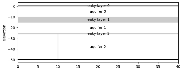
Plot the wells in a cross-section.
fig, ax = plt.subplots(1, 1, figsize=(8, 3))
ml4.plots.xsection(xy=[(0, 20), (0, -20)], labels=True, ax=ax)
for w in ws.wlist:
    for ilay in w.layers:
        ax.plot([w.yc, w.yc], [ml4.aq.zaqtop[ilay], ml4.aq.zaqbot[ilay]], "k-")
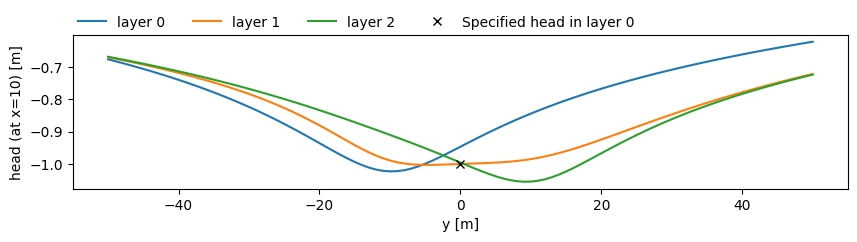
Plot a cross section of the head along y, showing all layers, and showing that the head in layer 0 runs through -1, the head we specified in the TargetHeadWellString.
y = np.linspace(-50, 50, 101)
x = ws.xcp * np.ones_like(y)
h4 = ml4.headalongline(x, y)

ilay = 0
plt.figure(figsize=(10, 2))
for ilay in range(ml4.aq.naq):
    plt.plot(y, h4[ilay], "-", label=f"layer {ilay}")
plt.plot(ws.ycp, ws.hcp, "kx", label="Specified head in layer 0")
plt.ylabel("head (at x=10) [m]")
plt.xlabel("y [m]")
plt.legend(loc=(0, 1), frameon=False, ncol=4);
Get total well discharge per layer
ws.discharge()
array([ 0. , 319.12051516, 1382.45288111])
Or per well, per layer
ws.discharge_per_well() # shape : (nlay, nwells)
array([[   0.        ,    0.        ],
       [ 319.12051516,    0.        ],
       [   0.        , 1382.45288111]])
Show that head inside the wells is equal:
ws.wlist[0].headinside(), ws.wlist[1].headinside()
(array([-4.08198052]), array([-4.08198052]))
The TargetHeadWellString element also has a headinside() method that returns a
single value (since the head inside must be equal).
ws.headinside()
np.float64(-4.081980524341912)
Test first well screened in two layers#
Test a TargetHeadWellString when the first well is screened in two layers.
lcp = 1
ml5 = tfs.ModelMaq(kaq=kaq, c=c, z=z, topboundary="semi", hstar=0)
ws = tfs.TargetHeadWellString(
    ml5,
    xy=[(0, -10), (0, 10)],
    rw=0.1,
    layers=[(0, 1), (2,)],
    res=0.0,
    hcp=-1,
    xcp=10,
    ycp=0,
    lcp=lcp,
)
ml5.solve()
Number of elements, Number of equations: 2 , 3
.
.

solution complete
fig, ax = plt.subplots(1, 1, figsize=(8, 3))
ml5.plots.xsection(xy=[(0, 20), (0, -20)], labels=True, ax=ax)
for w in ws.wlist:
    for ilay in w.layers:
        ax.plot([w.yc, w.yc], [ml5.aq.zaqtop[ilay], ml5.aq.zaqbot[ilay]], "k-")
y = np.linspace(-50, 50, 101)
x = ws.xcp * np.ones_like(y)
h5 = ml5.headalongline(x, y)

ilay = lcp
plt.figure(figsize=(10, 2))
for ilay in range(ml5.aq.naq):
    plt.plot(y, h5[ilay], "-", label=f"layer {ilay}")
plt.plot(ws.ycp, ws.hcp, "kx", label="Specified head in layer 0")
plt.ylabel("head (at x=10) [m]")
plt.xlabel("y [m]")
plt.legend(loc=(0, 1), frameon=False, ncol=4);
Compare the heads inside the wells
ws.wlist[0].headinside(), ws.wlist[1].headinside()
(array([-2.11729345, -2.11729345]), array([-2.11729345]))
ws.headinside()
np.float64(-2.117293450038338)
Compute the head at the target point, this should be equal to the specified head in the layer we entered.
ml5.head(xcp, ycp)
array([-0.94686224, -1. , -0.99561487])
HeadWellString with resistance#
Test the result when we add resistance to the wells.
ml = tfs.ModelMaq(kaq=kaq, c=c, z=z, topboundary="semi", hstar=0)
hws = tfs.HeadWellString(ml, xy=[(0, -10), (0, 10)], rw=0.1, res=0.1, layers=[0], hw=-2)
ml.solve()
Number of elements, Number of equations: 2 , 2
.
.

solution complete
The head inside the well should be equal to the specified head.
hws.headinside()
np.float64(-1.9999999999999996)
hws.wlist[0].headinside(), hws.wlist[1].headinside()
(array([-2.]), array([-2.]))
TargetHeadWellString with resistance#
Test a TargetHeadWellString with resistance.
lcp = 1
ml = tfs.ModelMaq(kaq=kaq, c=c, z=z, topboundary="semi", hstar=0)
thw = tfs.TargetHeadWellString(
    ml,
    xy=[(0, -10), (0, 10)],
    rw=0.1,
    layers=[(1,), (2,)],
    res=0.01,
    hcp=-1,
    xcp=10,
    ycp=0,
    lcp=lcp,
)
ml.solve()
Number of elements, Number of equations: 2 , 2
.
.

solution complete
Check that the head inside the well is equal.
thw.headinside()
np.float64(-2.60121594557672)
thw.wlist[0].headinside(), thw.wlist[1].headinside()
(array([-2.60121595]), array([-2.60121595]))
Verify that the head at the target point is met.
ml.head(thw.xcp, thw.ycp)
array([-0.53012579, -1. , -0.99114328])