Radial Collector Wells#
This notebook contains multi-layer solutions of examples in ‘Multilayer Analytic Element Modeling of Radial Collector Wells’
import numpy as np

import timflow.steady as tfs
Example 1#
k = 150  # hydraulic conductivity, m/d
z = [24, 16, 11, 7, 5, 4.05, 3.45, 3.15, 2.85, 2.55, 1.95, 1, 0]
kzoverkh = 1
layerw = 7
Qw = 12_000  # discharge of well, m^3/d
L = 60  # length of well, m
rw = 0.15  # radius of well, m
nls = 10  # number of (equally sized) line-sinks
xr, yr, hr = 60, 0, 24  # coordinates and head at reference point
#
xy = np.array(
    list(zip(np.linspace(-L / 2, L / 2, nls + 1), np.zeros(nls + 1), strict=False))
)
xyalt = np.zeros((nls, 4))  # specify begin and end of each line-sink
xyalt[:, 0] = xy[:-1, 0]
xyalt[:, 1] = xy[:-1, 1]
xyalt[:, 2] = xy[1:, 0]
xyalt[:, 3] = xy[1:, 1]
ml = tfs.Model3D(kaq=k, z=z, kzoverkh=kzoverkh)
w = tfs.CollectorWell(model=ml, xy=xy, Qw=Qw, layers=layerw, rw=rw)
rf = tfs.Constant(model=ml, xr=xr, yr=yr, hr=hr, layer=0)
ml.solve()
Number of elements, Number of equations: 2 , 11
.
.

solution complete
print("xcp, ycp, head in control points")
for i in range(nls):
    ls = w.lslist[i]
    print(ls.xc[0], ls.yc[0], ml.head(ls.xc[0], ls.yc[0], layers=layerw))
xcp, ycp, head in control points
-27.0 0.15 22.345373252961544
-21.0 0.15 22.34537325296192
-15.0 0.15 22.345373252962016
-9.0 0.15 22.3453732529621
-3.0 0.15 22.345373252961714
3.0 0.15 22.34537325296109
9.0 0.15 22.345373252962144
15.0 0.15 22.345373252961974
21.0 0.15 22.34537325296048
27.0 0.15 22.34537325296147
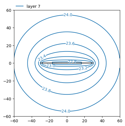
print(f"head in top layer at center of well {ml.head(0, 0, layers=0):.2f} m")
head in top layer at center of well 23.42 m
ml.plots.contour(
    win=[-60, 60, -60, 60],
    ngr=50,
    layers=7,
    levels=np.arange(20, 24.1, 0.2),
    decimals=1,
)
<Axes: >
ml = tfs.Model3D(kaq=k, z=z, kzoverkh=kzoverkh)
w = tfs.CollectorWell(model=ml, xy=xyalt, Qw=Qw, layers=layerw, rw=rw)
rf = tfs.Constant(model=ml, xr=xr, yr=yr, hr=hr, layer=0)
ml.solve()
Number of elements, Number of equations: 2 , 11
.
.

solution complete
ml.plots.contour(
    win=[-60, 60, -60, 60],
    ngr=50,
    layers=7,
    levels=np.arange(20, 24.1, 0.2),
    decimals=1,
);
print("xcp, ycp, head in control points")
for i in range(nls):
    ls = w.lslist[i]
    print(ls.xc[0], ls.yc[0], ml.head(ls.xc[0], ls.yc[0], layers=layerw))
xcp, ycp, head in control points
-27.0 0.15 22.345373252961544
-21.0 0.15 22.34537325296192
-15.0 0.15 22.345373252962016
-9.0 0.15 22.3453732529621
-3.0 0.15 22.345373252961714
3.0 0.15 22.34537325296109
9.0 0.15 22.345373252962144
15.0 0.15 22.345373252961974
21.0 0.15 22.34537325296048
27.0 0.15 22.34537325296147
print(f"head in top layer at center of well {ml.head(0, 0, layers=0):.2f} m")
head in top layer at center of well 23.42 m
Example 2#
rcaisson = 3 # radius caisson, m
xr, yr, hr = 100, 0, 24 # coordinates and head at reference point, m
Qw = 60_000 # discharge of well, m^3/d
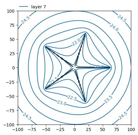
narms = 5
ml = tfs.Model3D(kaq=k, z=z, kzoverkh=kzoverkh)
w = tfs.RadialCollectorWell(
model=ml,
x=0,
y=0,
L=60,
rcaisson=rcaisson,
Qw=Qw,
narms=narms,
rw=rw,
nls=nls,
layers=7,
)
rf = tfs.Constant(model=ml, xr=xr, yr=yr, hr=hr, layer=0)
ml.solve()
ml.plots.contour(
win=[-100, 100, -100, 100],
ngr=101,
layers=7,
levels=np.arange(21, 30, 0.5),
decimals=1,
);
Number of elements, Number of equations: 2 , 51
.
.

solution complete
w.lslist[0]
River from (3.0, 0.0) to (9.0, 0.0)
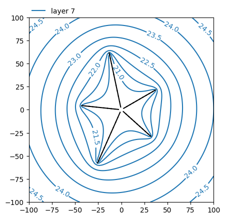
rcaisson = 3  # radius caisson, m
xr, yr, hr = 100, 0, 24  # coordinates and head at reference point, m
Qw = 60_000  # discharge of well, m^3/d
narms = 5

ml = tfs.Model3D(kaq=k, z=z, kzoverkh=kzoverkh)
w = tfs.RadialCollectorWell(
    model=ml,
    x=0,
    y=0,
    L=[40, 60, 40, 60, 40],
    angle=30,
    rcaisson=rcaisson,
    Qw=Qw,
    narms=narms,
    rw=rw,
    nls=nls,
    layers=7,
)
rf = tfs.Constant(model=ml, xr=xr, yr=yr, hr=hr, layer=0)
ml.solve()
ml.plots.contour(
    win=[-100, 100, -100, 100],
    ngr=101,
    layers=7,
    levels=np.arange(21, 30, 0.5),
    decimals=1,
);
Number of elements, Number of equations: 2 , 51
.
.

solution complete
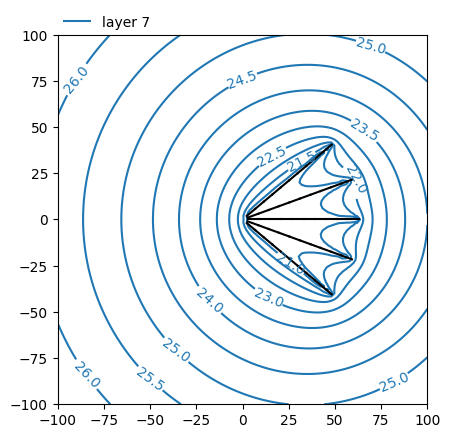
rcaisson = 3  # radius caisson, m
xr, yr, hr = 100, 0, 24  # coordinates and head at reference point, m
Qw = 60_000  # discharge of well, m^3/d
narms = 5

ml = tfs.Model3D(kaq=k, z=z, kzoverkh=kzoverkh)
w = tfs.RadialCollectorWell(
    model=ml,
    x=0,
    y=0,
    L=60,
    angle=[-40, -20, 0, 20, 40],
    rcaisson=rcaisson,
    Qw=Qw,
    narms=narms,
    rw=rw,
    nls=nls,
    layers=7,
)
rf = tfs.Constant(model=ml, xr=xr, yr=yr, hr=hr, layer=0)
ml.solve()
ml.plots.contour(
    win=[-100, 100, -100, 100],
    ngr=101,
    layers=7,
    levels=np.arange(21, 30, 0.5),
    decimals=1,
);
Number of elements, Number of equations: 2 , 51
.
.

solution complete
rcaisson = 3 # radius caisson, m
xr, yr, hr = 100, 0, 24 # coordinates and head at reference point, m
Qw = 60_000 # discharge of well, m^3/d
narms = 5
ml = tfs.Model3D(kaq=k, z=z, kzoverkh=kzoverkh)
w = tfs.RadialCollectorWell(
model=ml,
x=0,
y=0,
L=60,
rcaisson=rcaisson,
Qw=Qw,
narms=narms,
rw=rw,
nls=nls,
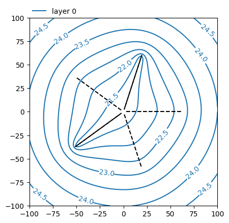
layers=[7, 0, 7, 0, 7], # just for illustration purposes
)
rf = tfs.Constant(model=ml, xr=xr, yr=yr, hr=hr, layer=0)
ml.solve()
# contour in layer 0
ax = ml.plots.contour(
win=[-100, 100, -100, 100],
ngr=101,
layers=0,
levels=np.arange(21, 30, 0.5),
decimals=1,
)
# plot arms in layer 0 with dashed lines
ax = w.plot(ax=ax, layer=7, ls="dashed")
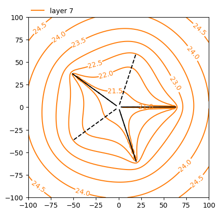
# contour in layer 7
ax = ml.plots.contour(
win=[-100, 100, -100, 100],
ngr=101,
layers=7,
levels=np.arange(21, 30, 0.5),
decimals=1,
color="C1",
)
# plot arms in layer 0 with dashed lines
w.plot(ax=ax, layer=0, ls="dashed");
Number of elements, Number of equations: 2 , 51
.
.

solution complete
headinside = []
print("head in collector well:", w.headinside())
for i in range(w.nls):
    ls = w.lslist[i]
    headinside.append(ml.head(ls.xc[0], ls.yc[0], layers=ls.layers[0]))
headinside = np.array(headinside)
assert np.allclose(headinside[1:], headinside[0])
head in collector well: 21.056785021938442
Q_arms = w.discharge_per_arm()
print("discharge of each arm: ", Q_arms)
discharge of each arm:  [ 9728.78096301 15684.65174892  9165.09929385 15691.03050211
  9730.4374921 ]
Note that the discharge of arms 0, 2, 4, and the discharges of arms 1, 3 are not exactly equal, even though you may expect that from symmetry. This is the case because the control points are put a horizontal distance rw away along each arm, always on the left side when going from the point closest to the caisson to the end point.