How-to: Select a Model

This guide explains the differences between the four model classes in timflow.steady: ModelMaq, Model3D, Model and ModelXsection. Understanding these differences will help you choose the right model type for your groundwater flow problem.

import timflow.steady as tfs

ModelMaq

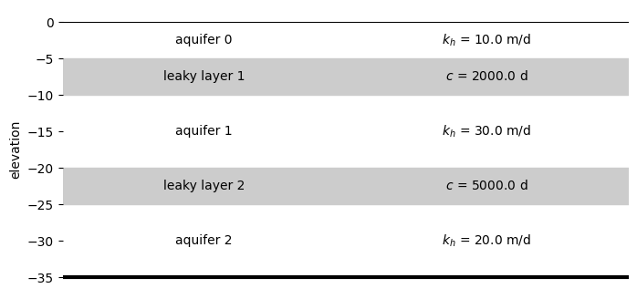
ModelMaq is a model consisting of a regular sequence of aquifer - leaky layer - aquifer - leaky layer, aquifer, etc. The top of the system can be either an aquifer or a leaky layer. The head is computed in all aquifer layers only.

ml = tfs.ModelMaq(z=[0, -5, -10, -20, -25, -35], kaq=[10, 30, 20], c=[2000, 5000])

Show aquifer summary

ml.aquifer_summary()

		layer	layer_type	H	k_h	c
	#
background	0	0	aquifer	5	10.0	NaN
	1	1	leaky layer	5	NaN	2000.0
	2	1	aquifer	10	30.0	NaN
	3	2	leaky layer	5	NaN	5000.0
	4	2	aquifer	10	20.0	NaN

The figure below illustrates a ModelMaq example with three aquifers and two leaky layers:

ax = ml.plots.xsection(params=True, labels=True, units={"k": "m/d", "c": "d"})
ax.set_frame_on(False)

Model3D

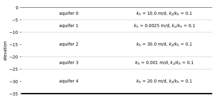
Model3D is a model consisting of a stack of aquifer layers. The resistance between the aquifer layers is computed as the resistance from the middle of one layer to the middle of the next layer. Vertical anisotropy can be specified. The system may be bounded on top by a leaky layer.

ml = tfs.Model3D(
    z=[0, -5, -10, -20, -25, -35], kaq=[10, 0.0025, 30, 0.001, 20], kzoverkh=0.1
)

Show aquifer summary

ml.aquifer_summary()

		layer	layer_type	H	k_h	c	kzoverkh
	#
background	0	0	aquifer	5	10.0	NaN	0.1
	1	1	aquifer	5	0.0025	10002.5	0.1
	2	2	aquifer	10	30.0	10001.666667	0.1
	3	3	aquifer	5	0.001	25001.666667	0.1
	4	4	aquifer	10	20.0	25002.5	0.1

The figure below shows a Model3D example consisting of five layers all treated as aquifers with a vertical anisotropy of 0.1:

ax = ml.plots.xsection(params=True, labels=True, units={"k": "m/d", "c": "d"})
ax.set_frame_on(False)

Model

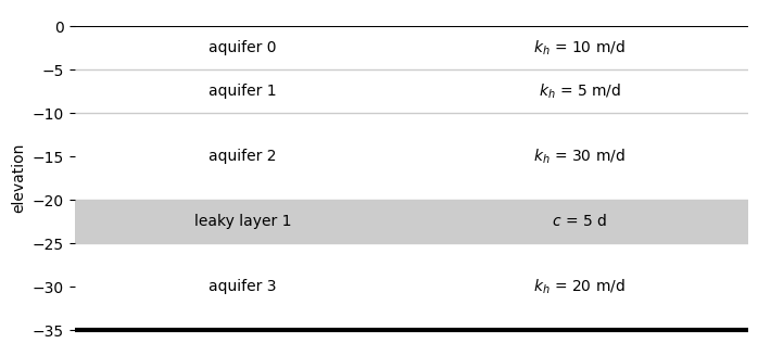
Model is a model consisting of an arbitrary sequence of leaky layers and aquifers. The resistance between all aquifers needs to be specified by the user. This is the most general option, but requires a bit more input.

ml = tfs.Model(
    z=[0, -5, -10, -20, -25, -35],
    kaq=[10, 5, 30, 20],
    c=[2, 5, 2000],
    npor=[0.3, 0.3, 0.3, 0.3, 0.3],
    ltype=["a", "a", "a", "l", "a"],
)

The figure below illustrates a Model example with four aquifers and one leaky layer:

ax = ml.plots.xsection(params=True, labels=True, units={"k": "m/d", "c": "d"})
ax.set_frame_on(False)

XsectionModel

XsectionModel is a special model class for building cross-section models. The only parameter you can pass to ModelXsection is the number of layers, which must be equal for all sections.

ml = tfs.ModelXsection(naq=2)