Building Pit#
This example demonstrates the modeling of a building pit with dewatering wells using timflow. The model calculates groundwater flow towards the pit and evaluates the effectiveness of dewatering strategies by computing total discharge and drawdown distances.
Note
It is highly recommended to use the BuildingPit element if you want to
implement different layer properties inside the building pit as compared to the rest of
the aquifer. Adding barriers, e.g. LeakyWalls, around an inhomogeneity will
not work.
import matplotlib.pyplot as plt
import numpy as np

import timflow.steady as tfs
Parameters#
Define some aquifer parameters
kh = 2.0  # m/day
f_ani = 1 / 10  # anisotropy factor
kv = f_ani * kh
ctop = 800.0  # resistance top leaky layer in days
Define aquifer top and bottom, the depth of the sheetpile wall and the position of the dewatering wells.
ztop = 0.0  # surface elevation
z_well = -13.0  # end depth of the wellscreen
z_dw = -15.0  # bottom elevation of sheetpile wall
z_extra = z_dw - 15.0  # extra layer
zbot = -60.0  # bottom elevation of the model
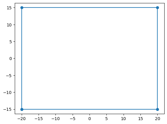
Size of the building pit, and the required drawdown at the center of the building pit.
length = 40.0  # length building pit in m
width = 30.0  # width building pit in m

h_bem = -6.21  # m
offset = 5.0  # distance groundwater extraction element from sheetpiles in m
xy = [
    (-length / 2, -width / 2),
    (length / 2, -width / 2),
    (length / 2, width / 2),
    (-length / 2, width / 2),
    (-length / 2, -width / 2),
]
Plot the building pit
(p2,) = plt.plot(*np.array(xy).T, "o-")
plt.axis("equal")
plt.show()
Model#
Set up a model
z = np.array([ztop + 1, ztop, z_dw, z_dw, z_extra, z_extra, zbot])
dz = z[1::2] - z[2::2]
kh_arr = kh * np.ones(dz.shape)
Resistances of the top confining layer and aquitards
c = np.r_[np.array([ctop]), dz[:-1] / (2 * kv) + dz[1:] / (2 * kv)]
Build model, solve, and calculate total discharge and distance to the 5 cm drawdown contour.
ml = tfs.ModelMaq(kaq=kh_arr, z=z, c=c, topboundary="semi", hstar=0.0)

layers = np.arange(np.sum(z_dw <= ml.aq.zaqbot))
last_lay_dw = layers[-1]

inhom = tfs.BuildingPitMaq(
    ml,
    xy,
    kaq=kh_arr,
    z=z[1:],
    topboundary="conf",
    c=c[1:],
    order=4,
    ndeg=3,
    layers=layers,
)

tfs.River(
    ml,
    x1=-length / 2 + offset,
    y1=width / 2 - offset,
    x2=length / 2 - offset,
    y2=width / 2 - offset,
    hls=h_bem,
    layers=np.arange(last_lay_dw + 1),
)
tfs.River(
    ml,
    x1=-length / 2 + offset,
    y1=0,
    x2=length / 2 - offset,
    y2=0,
    hls=h_bem,
    layers=np.arange(last_lay_dw + 1),
)
tfs.River(
    ml,
    x1=-length / 2 + offset,
    y1=-width / 2 + offset,
    x2=length / 2 - offset,
    y2=-width / 2 + offset,
    hls=h_bem,
    layers=np.arange(last_lay_dw + 1),
)

# ml.solve_mp(nproc=2)
ml.solve()

Qtot = 0.0

for e in ml.elementlist:
    if e.name == "River":
        Qtot += e.discharge()

print("\nDischarge =", np.round(Qtot.sum(), 2), "m^3/day")

y = np.linspace(-width / 2 - 25, width / 2 + 1100, 201)
hl = ml.headalongline(np.zeros(201), y, layers=[0])
y_5cm = np.interp(
    -0.05, ml.headalongline(np.zeros(201), y, layers=0).squeeze(), y, right=np.nan
)
print("Distance to 5 cm drawdown contour =", np.round(y_5cm, 2), "m")
Number of elements, Number of equations: 21 , 124
.
.
.
.
.
.
.
.
.
.
.
.
.
.
.
.
.
.
.
.
.

solution complete

Discharge = 88.1 m^3/day
Distance to 5 cm drawdown contour = 301.43 m
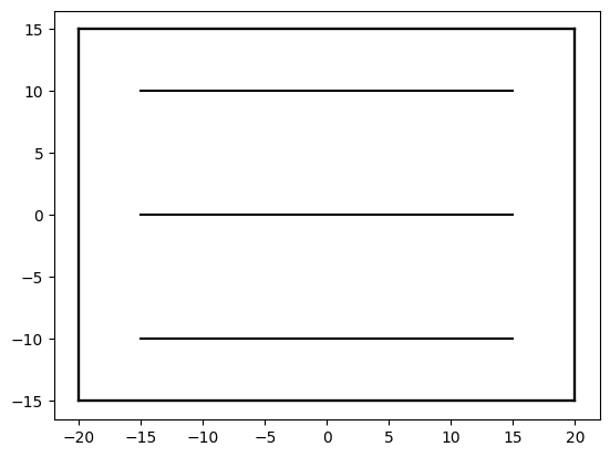
Plot an overview of the model
ml.plots.topview()
<Axes: >
Visualizations
x = np.linspace(0.0, length / 2 + 1100, 201)
hl = ml.headalongline(x, np.zeros(201), layers=[last_lay_dw, last_lay_dw + 1])
fig, ax = plt.subplots(1, 1, figsize=(10, 3))
ax.plot(x, hl[0].squeeze(), label="head layer {}".format(last_lay_dw))
ax.plot(x, hl[1].squeeze(), label="head layer {}".format(last_lay_dw + 1))
ax.axhline(-0.05, color="r", linestyle="dashed", lw=0.75, label="-0.05 m")
ax.axhline(-0.5, color="k", linestyle="dashed", lw=0.75, label="-0.5 m")
ax.set_xlabel("x (m)")
ax.set_ylabel("head (m)")
ax.legend(loc="best")
ax.grid(True)

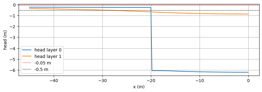
x = np.linspace(-length / 2 - 25, 0.0, 201)
hl = ml.headalongline(x, np.zeros(201), layers=[last_lay_dw, last_lay_dw + 1])
fig, ax = plt.subplots(1, 1, figsize=(10, 3))

ax.plot(x, hl[0].squeeze(), label="head layer {}".format(last_lay_dw))
ax.plot(x, hl[1].squeeze(), label="head layer {}".format(last_lay_dw + 1))
ax.axhline(-0.05, color="r", linestyle="dashed", lw=0.75, label="-0.05 m")
ax.axhline(-0.5, color="k", linestyle="dashed", lw=0.75, label="-0.5 m")
ax.set_xlabel("x (m)")
ax.set_ylabel("head (m)")
ax.legend(loc="best")
ax.grid(True)
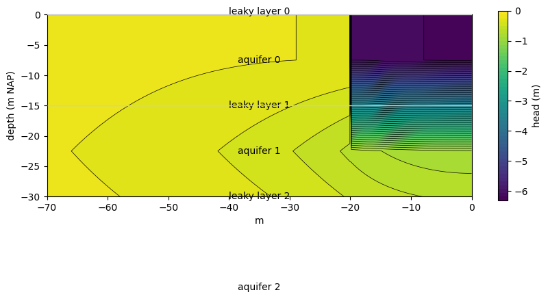
Plot cross-section around the sheetpile wall
xoffset = 50
zoffset = 15
x1, x2, y1, y2 = [-length / 2 - xoffset, 0.0, 0, 0]
nudge = 1e-6
n = 301
# plot head contour cross-sections
h = ml.headalongline(
    np.linspace(x1 + nudge, x2 - nudge, n),
    np.linspace(y1 + nudge, y2 - nudge, n),
)
L = np.sqrt((x2 - x1) ** 2 + (y2 - y1) ** 2)
xg = np.linspace(0, L, n) + x1

zg = 0.5 * (ml.aq.zaqbot + ml.aq.zaqtop)
zg = np.hstack((ml.aq.zaqtop[0], zg, ml.aq.zaqbot[-1]))
h = np.vstack((h[0], h, h[-1]))

ymid = np.mean([y1, y2])
levels = np.linspace(h_bem - 0.1, -0.0, 51)

fig, ax = plt.subplots(1, 1, figsize=(10, 6))
ax.set_aspect("equal")
ml.plots.xsection(
    xy=[(x1, ymid), (x2, ymid)],
    ax=ax,
    horizontal_axis="x",
    labels=True,
    zorder=10,
)
cf = ax.contourf(xg, zg, h, levels)
cs = ax.contour(xg, zg, h, levels, colors="k", linewidths=0.5)
ax.set_ylim(z_dw - zoffset, z_dw + zoffset)
ax.set_ylabel("depth (m NAP)")
ax.set_xlabel("m")

cb = plt.colorbar(cf, ax=ax, shrink=0.6)
cb.set_label("head (m)")
cb.set_ticks(np.arange(-6, 0.1, 1))
Model 2: Add more layers#
Add more layers to the model to get a more accurate solution of the flow towards the building pit.
n = 11 # number of layers around bottom of sheetpile wall
# Calculate thickness of each sublayer above and below the sheetpile wall
dz_i_top = (z_well - z_dw) / np.sum(np.arange(n + 1))
dz_i_bot = (z_dw - z_extra) / np.sum(np.arange(2 * n + 1))

# Generate cumulative depths for sublayers above and below the wall
z_layers_top = np.cumsum(np.arange(n) * dz_i_top)
z_layers_bot = np.cumsum(np.arange(2 * n) * dz_i_bot)

# Combine sublayer depths into a single array for the model
zgr = np.r_[z_dw + z_layers_top[::-1], (z_dw - z_layers_bot)[1:]]

# Build full array of layer boundaries for the model
z4 = np.r_[
    np.array([ztop + 1, ztop, z_well, z_well]),
    np.repeat(zgr, 2, 0),
    z_extra,
    z_extra,
    zbot,
]

# Calculate thicknesses and hydraulic conductivities for each layer
dz4 = z4[1:-1:2] - z4[2::2]
kh_arr = kh * np.ones(dz4.shape)

# Calculate resistance for each layer
c = np.r_[np.array([ctop]), dz4[:-1] / (2 * kv) + dz4[1:] / (2 * kv)]

# Set hydraulic conductivity of the top layer to a very low value
kh_arr2 = kh_arr.copy()
kh_arr2[0] = 1e-5
Build model, solve, and calculate total discharge and distance to the 5 cm drawdown contour.
ml = tfs.ModelMaq(kaq=kh_arr, z=z4, c=c, topboundary="semi", hstar=0.0)

layers = np.arange(np.sum(z_dw <= ml.aq.zaqbot))
last_lay_dw = layers[-1]
inhom = tfs.BuildingPitMaq(
    ml,
    xy,
    kaq=kh_arr2,
    z=z4[1:],
    topboundary="conf",
    c=c[1:],
    order=4,
    ndeg=3,
    layers=layers,
)

wlayers = np.arange(np.sum(-14 <= ml.aq.zaqbot))
wlayers = wlayers[1:]

tfs.River(
    ml,
    x1=-length / 2 + offset,
    y1=width / 2 - offset,
    x2=length / 2 - offset,
    y2=width / 2 - offset,
    hls=h_bem,
    layers=wlayers,
)
tfs.River(
    ml,
    x1=-length / 2 + offset,
    y1=0,
    x2=length / 2 - offset,
    y2=0,
    hls=h_bem,
    layers=wlayers,
    order=5,
)
tfs.River(
    ml,
    x1=-length / 2 + offset,
    y1=-width / 2 + offset,
    x2=length / 2 - offset,
    y2=-width / 2 + offset,
    hls=h_bem,
    layers=wlayers,
)

# ml.solve_mp(nproc=2)
ml.solve()

Qtot_ml = 0.0

for e in ml.elementlist:
    if e.name == "River":
        Qtot_ml += e.discharge()

print("\nDischarge =", np.round(Qtot_ml.sum(), 2), "m^3/day")

y = np.linspace(-width / 2 - 25, width / 2 + 1100, 201)
hl = ml.headalongline(np.zeros(201), y, layers=[0])
y_5cm_ml = np.interp(
    -0.05, ml.headalongline(np.zeros(201), y, layers=0).squeeze(), y, right=np.nan
)
print("Distance to 5 cm drawdown contour =", np.round(y_5cm_ml, 2), "m")
Number of elements, Number of equations: 21 , 1425
.
.
.
.
.
.
.
.
.
.
.
.
.
.
.
.
.
.
.
.
.

solution complete

Discharge = 210.29 m^3/day
Distance to 5 cm drawdown contour = 500.64 m
last_lay_dw = layers[-1]
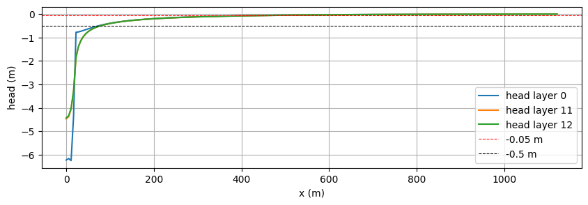
x = np.linspace(0.0, length / 2 + 1100, 201)
hl = ml.headalongline(x, np.zeros(201), layers=[0, last_lay_dw, last_lay_dw + 1])
fig, ax = plt.subplots(1, 1, figsize=(10, 3))

ax.plot(x, hl[0].squeeze(), label="head layer 0")
ax.plot(x, hl[1].squeeze(), label="head layer {}".format(last_lay_dw))
ax.plot(x, hl[2].squeeze(), label="head layer {}".format(last_lay_dw + 1))
ax.axhline(-0.05, color="r", linestyle="dashed", lw=0.75, label="-0.05 m")
ax.axhline(-0.5, color="k", linestyle="dashed", lw=0.75, label="-0.5 m")
ax.set_xlabel("x (m)")
ax.set_ylabel("head (m)")
ax.legend(loc="best")
ax.grid(True)
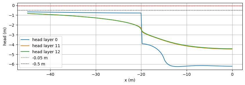
x = np.linspace(-length / 2 - 25, 0.0, 201)
hl = ml.headalongline(x, np.zeros(201), layers=[0, last_lay_dw, last_lay_dw + 1])
fig, ax = plt.subplots(1, 1, figsize=(10, 3))

ax.plot(x, hl[0].squeeze(), label="head layer 0")
ax.plot(x, hl[1].squeeze(), label="head layer {}".format(last_lay_dw))
ax.plot(x, hl[2].squeeze(), label="head layer {}".format(last_lay_dw + 1))
ax.axhline(-0.05, color="r", linestyle="dashed", lw=0.75, label="-0.05 m")
ax.axhline(-0.5, color="k", linestyle="dashed", lw=0.75, label="-0.5 m")
ax.set_xlabel("x (m)")
ax.set_ylabel("head (m)")
ax.legend(loc="best")
ax.grid(True)
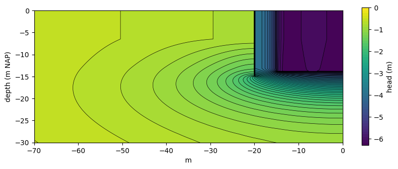
Plot head contours in a vertical cross-section around the sheetpile wall.
xoffset = 50
zoffset = 15
x1, x2, y1, y2 = [-length / 2 - xoffset, 0.0, 0, 0]
nudge = 1e-6
n = 301
# plot head contour cross-sections
h = ml.headalongline(
    np.linspace(x1 + nudge, x2 - nudge, n), np.linspace(y1 + nudge, y2 - nudge, n)
)
L = np.sqrt((x2 - x1) ** 2 + (y2 - y1) ** 2)
xg = np.linspace(0, L, n) + x1

zg = 0.5 * (ml.aq.zaqbot + ml.aq.zaqtop)
zg = np.hstack((ml.aq.zaqtop[0], zg, ml.aq.zaqbot[-1]))
h = np.vstack((h[0], h, h[-1]))
levels = np.linspace(h_bem - 0.1, -0.0, 51)

fig, ax = plt.subplots(1, 1, figsize=(10, 6))
ax.set_aspect("equal")
ml.plots.xsection(xy=[(x1, ymid), (x2, ymid)], ax=ax, labels=False, horizontal_axis="x")
cf = ax.contourf(xg, zg, h, levels)
cs = ax.contour(xg, zg, h, levels, colors="k", linewidths=0.5)
ax.set_ylim(z_dw - zoffset, z_dw + zoffset)
ax.set_ylabel("depth (m NAP)")
ax.set_xlabel("m")

cb = plt.colorbar(cf, ax=ax, shrink=0.6)
cb.ax.set_ylabel("head (m)")
cb.set_ticks(np.arange(-6, 0.1, 1))
Note the difference between the computed discharge between the model with only a few layers and the model with very fine layers.
print("Number of layers                  |  N=3  |  N=35 | unit")
print("-" * 56)
print(
    f"Discharge from building pit       | {Qtot.sum():>5.1f} "
    f"| {Qtot_ml.sum():>5.1f} | m^3/d"
)
print(f"Distance to 5 cm drawdown contour | {y_5cm:>5.1f} | {y_5cm_ml:>5.1f} | m")
Number of layers                  |  N=3  |  N=35 | unit
--------------------------------------------------------
Discharge from building pit       |  88.1 | 210.3 | m^3/d
Distance to 5 cm drawdown contour | 301.4 | 500.6 | m