Inhomogeneities with Model3D

Consider a multi-layer aquifer system that contains one inhomogeneity. Inside the inhomogeneity the transmissivity of the top aquifer is much lower and the transmissivity of the bottom aquifer is much higher than outside the inhomogeneity. A well is located in the top aquifer inside the inhomogeneity (the black dot).

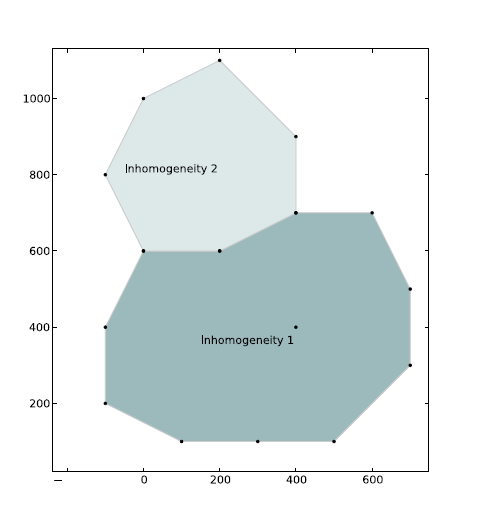
The layout of the inhomogeneity is shown in the figure below. Aquifer properties are specified in the code.

Figure 1: Layout of elements for this exercise. A well is located inside inhomogeneity 1.

import matplotlib.pyplot as plt
import numpy as np

import timflow.steady as tfs

plt.rcParams["figure.figsize"] = (6, 6)

ml = tfs.Model3D(kaq=10, z=[20, 10, 0], kzoverkh=0.02)
xy1 = [
    (0, 600),
    (-100, 400),
    (-100, 200),
    (100, 100),
    (300, 100),
    (500, 100),
    (700, 300),
    (700, 500),
    (600, 700),
    (400, 700),
    (200, 600),
]
p1 = tfs.PolygonInhom3D(
    ml,
    xy=xy1,
    kaq=2,
    z=[20, 10, 0],
    kzoverkh=0.002,
    topboundary="conf",
    order=5,
    ndeg=3,
)
rf = tfs.Constant(ml, xr=1000, yr=0, hr=40)
uf = tfs.Uflow(ml, slope=0.002, angle=-45)
w = tfs.Well(ml, xw=400, yw=400, Qw=500, rw=0.2, layers=0)
ml.solve()

Number of elements, Number of equations: 26 , 266
.
.
.
.
.
.
.
.
.
.
.
.
.
.
.
.
.
.
.
.
.
.
.
.
.
.

solution complete

Questions

Exercise 3a

What are the leakage factors of the background aquifer and the inhomogeneity?

print("Leakage factor of the background aquifer is:", ml.aq.lab)
print("Leakage factor of the inhomogeneity is:", p1.lab)

Leakage factor of the background aquifer is: [ 0. 50.]
Leakage factor of the inhomogeneity is: [  0.         158.11388301]

Exercise 3b

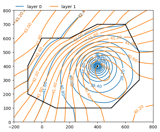
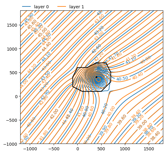
Make a contour plot of both aquifers.

ml.plots.contour(
    win=[-200, 800, 0, 800], ngr=50, layers=[0, 1], levels=20, labels=1, decimals=2
)

<Axes: >

ml.plots.contour(
    win=[-1200, 1800, -1000, 1800],
    ngr=50,
    layers=[0, 1],
    levels=50,
    labels=1,
    decimals=2,
)

<Axes: >

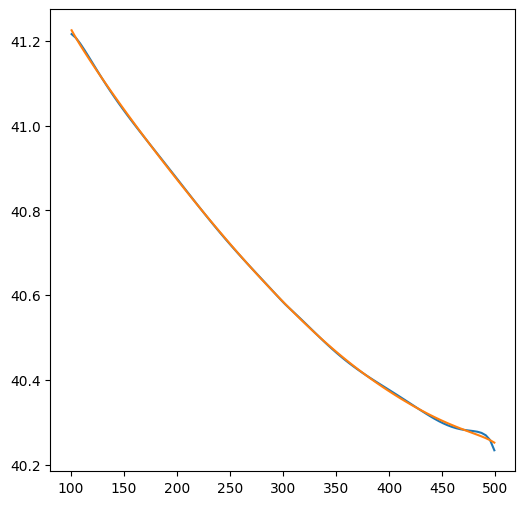
htop = ml.headalongline(np.linspace(101, 499, 100), 100 + 0.001 * np.ones(100))
hbot = ml.headalongline(np.linspace(101, 499, 100), 100 - 0.001 * np.ones(100))
plt.figure()
plt.plot(np.linspace(101, 499, 100), htop[0])
plt.plot(np.linspace(101, 499, 100), hbot[0])

[<matplotlib.lines.Line2D at 0x7232241dd310>]

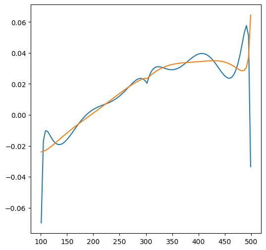
qtop = np.zeros(100)
qbot = np.zeros(100)
layer = 1
x = np.linspace(101, 499, 100)
for i in range(100):
    qx, qy = ml.disvec(x[i], 100 + 0.001)
    qtop[i] = qy[layer]
    qx, qy = ml.disvec(x[i], 100 - 0.001)
    qbot[i] = qy[layer]
plt.figure()
plt.plot(x, qtop)
plt.plot(x, qbot)

[<matplotlib.lines.Line2D at 0x72322407c7d0>]

Exercise 3c

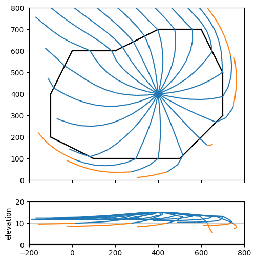
Create a 20-year capture zone for the well, starting the pathlines halfway the top aquifer. First create a contour plot with a cross-section below it.

axes = ml.plots.topview_and_xsection(win=[-200, 800, 0, 800])
ml.plots.plotcapzone(
    well=w, hstepmax=50, nt=20, zstart=15, tmax=20 * 365.25, orientation="both", ax=axes
)

.
.
.
.
.
.
.
.
.
.
.
.
.
.
.
.
.
.
.
.

array([<Axes: >, <Axes: ylabel='elevation'>], dtype=object)

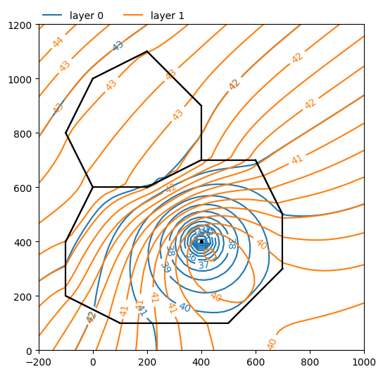
Two inhomogeneities

A second inhomogeneity is added, which shares part of its boundary with the first inhomogeneity. The aquifer properties for the inhomogeneity are provided in table 3. Inside this second inhomogeneity, the transmissivity of both the bottom aquifer and the resistance of the leaky layer are reduced. The input is now somewhat complicated. First the data of the two inhomgeneities is entered. Second, analytic elements are placed along the boundary of the inhomogeneity with MakeInhomPolySide. This routine places line elements along a string of points, but it requires that the aquifer data is the same on the left and right sides of the line. Hence, for this case we need to break the boundary up in three sections: One section with the background aquifer on one side and inhom1 on the other, one section with the background aquifer on one side and inhom2 on the other, and one section with inhom1 on one side and inhom2 on the other. The input file is a bit longer

Table 3: Inhomogeneity 2 data

Layer	\(k\) (m/d)	\(z_b\) (m)	\(z_t\)	\(c\) (days)
Aquifer 0	2	-20	0	-
Leaky Layer 1	-	-40	-20	50
Aquifer 1	8	-80	-40	-

ml = tfs.Model3D(kaq=10, z=[20, 10, 0], kzoverkh=0.02)
xy1 = [
    (0, 600),
    (-100, 400),
    (-100, 200),
    (100, 100),
    (300, 100),
    (500, 100),
    (700, 300),
    (700, 500),
    (600, 700),
    (400, 700),
    (200, 600),
]
p1 = tfs.PolygonInhom3D(
    ml,
    xy=xy1,
    kaq=2,
    z=[20, 10, 0],
    kzoverkh=0.002,
    topboundary="conf",
    order=5,
    ndeg=3,
)
xy2 = [
    (0, 600),
    (200, 600),
    (400, 700),
    (400, 900),
    (200, 1100),
    (0, 1000),
    (-100, 800),
]
p2 = tfs.PolygonInhom3D(
    ml,
    xy=xy2,
    kaq=20,
    z=[20, 10, 0],
    kzoverkh=0.05,
    topboundary="conf",
    order=5,
    ndeg=3,
)
rf = tfs.Constant(ml, xr=1000, yr=0, hr=40)
uf = tfs.Uflow(ml, slope=0.002, angle=-45)
w = tfs.Well(ml, xw=400, yw=400, Qw=500, rw=0.2, layers=0)
ml.solve()

Number of elements, Number of equations: 37 , 387
.
.
.
.
.
.
.
.
.
.
.
.
.
.
.
.
.
.
.
.
.
.
.
.
.
.
.
.
.
.
.
.
.
.
.
.
.

solution complete

ml.plots.contour(win=[-200, 1000, 0, 1200], ngr=50, layers=[0, 1], levels=20);