Cross-Sectional Models#
This notebook demonstrates how to build and solve cross-sectional (1D) models in timflow, including examples with strip inhomogeneities and infinitely long line elements.
import matplotlib.pyplot as plt
import numpy as np

import timflow.steady as tfs

plt.rcParams["figure.figsize"] = (4, 3)
plt.rcParams["figure.autolayout"] = True
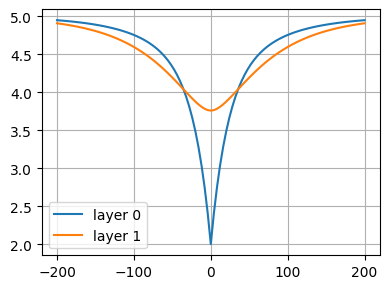
Two-layer model with head-specified line-sink#
Two-layer aquifer bounded on top by a semi-confined layer. Head above the semi-confining layer is 5. Head line-sink located at \(x=0\) with head equal to 2, cutting through layer 0 only.
ml = tfs.ModelMaq(
    kaq=[1, 2], z=[4, 3, 2, 1, 0], c=[1000, 1000], topboundary="semi", hstar=5
)
ls = tfs.River1D(ml, xls=0, hls=2, layers=0)
ml.solve()

x = np.linspace(-200, 200, 101)
h = ml.headalongline(x, np.zeros_like(x))
plt.plot(x, h[0], label="layer 0")
plt.plot(x, h[1], label="layer 1")
plt.legend(loc="best")
plt.grid()
Number of elements, Number of equations: 2 , 1
.
.

solution complete
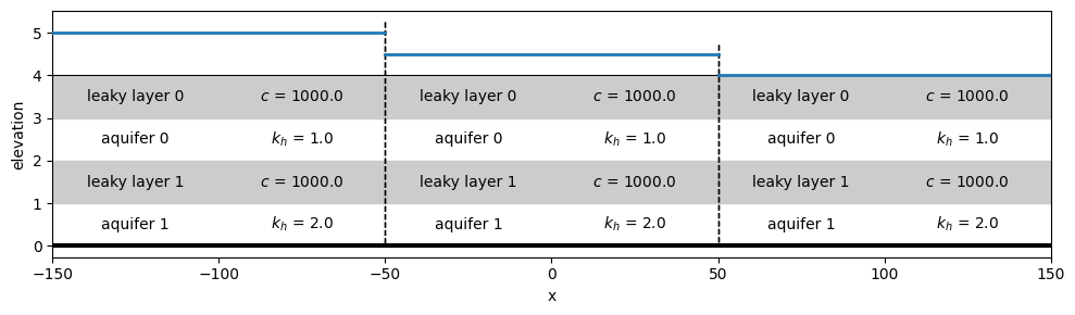
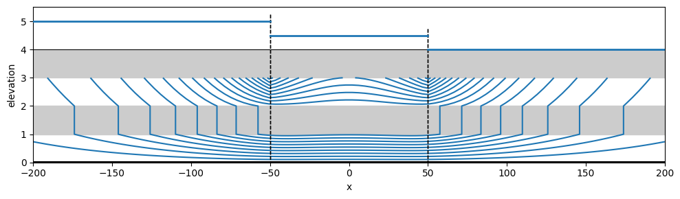
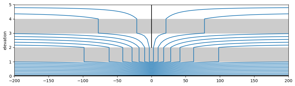
1D inhomogeneity#
Three strips with semi-confined conditions on top of all three
ml = tfs.ModelXsection(naq=2)
tfs.XsectionMaq(
    ml,
    x1=-np.inf,
    x2=-50,
    kaq=[1, 2],
    z=[4, 3, 2, 1, 0],
    c=[1000, 1000],
    npor=0.3,
    topboundary="semi",
    hstar=5,
)
tfs.XsectionMaq(
    ml,
    x1=-50,
    x2=50,
    kaq=[1, 2],
    z=[4, 3, 2, 1, 0],
    c=[1000, 1000],
    npor=0.3,
    topboundary="semi",
    hstar=4.5,
)
tfs.XsectionMaq(
    ml,
    x1=50,
    x2=np.inf,
    kaq=[1, 2],
    z=[4, 3, 2, 1, 0],
    c=[1000, 1000],
    npor=0.3,
    topboundary="semi",
    hstar=4,
)
ml.solve()
Number of elements, Number of equations: 7 , 8
.
.
.
.
.
.
.

solution complete
fig, ax = plt.subplots(1, 1, figsize=(10, 3))
ml.plots.xsection(xy=[(-150, 0), (150, 0)], ax=ax, params=True);
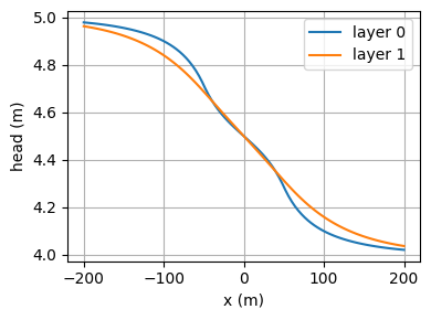
x = np.linspace(-200, 200, 101)
h = ml.headalongline(x, np.zeros(101))
plt.plot(x, h[0], label="layer 0")
plt.plot(x, h[1], label="layer 1")
plt.xlabel("x (m)")
plt.ylabel("head (m)")
plt.legend(loc="best")
plt.grid()
ml.plots.vcontoursf1D(x1=-200, x2=200, nx=100, levels=20, color="C0", figsize=(10, 3));
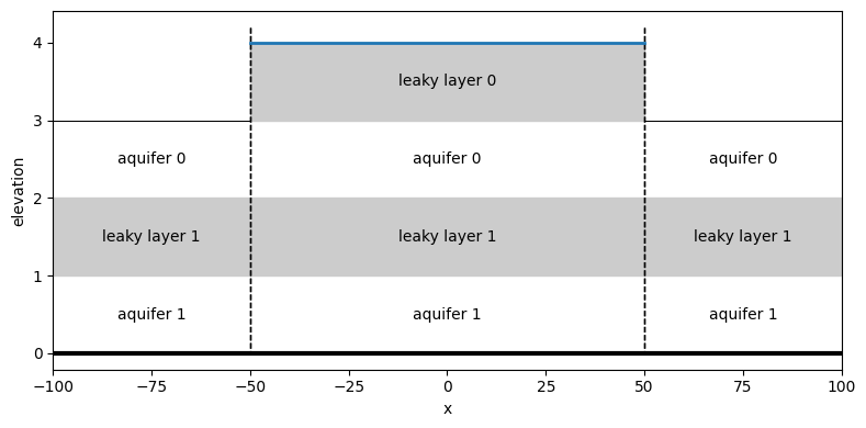
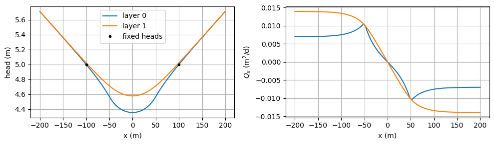
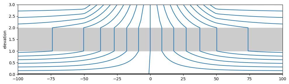
Three strips with semi-confined conditions at the top of the strip in the middle only. The head is specified in the strip on the left and in the strip on the right.
ml = tfs.ModelXsection(naq=2)
tfs.XsectionMaq(
    ml,
    x1=-np.inf,
    x2=-50,
    kaq=[1, 2],
    z=[3, 2, 1, 0],
    c=[1000],
    npor=0.3,
    topboundary="conf",
)
tfs.XsectionMaq(
    ml,
    x1=-50,
    x2=50,
    kaq=[1, 2],
    z=[4, 3, 2, 1, 0],
    c=[1000, 1000],
    npor=0.3,
    topboundary="semi",
    hstar=4,
)
tfs.XsectionMaq(
    ml,
    x1=50,
    x2=np.inf,
    kaq=[1, 2],
    z=[3, 2, 1, 0],
    c=[1000],
    npor=0.3,
    topboundary="conf",
)
rf1 = tfs.Constant(ml, -100, 0, 5)
rf2 = tfs.Constant(ml, 100, 0, 5)

ml.solve()

ml.plots.xsection(xy=[(-100, 0), (100, 0)]);
Number of elements, Number of equations: 7 , 10
.
.
.
.
.
.
.

solution complete
x = np.linspace(-200, 200, 101)
h = ml.headalongline(x, np.zeros_like(x))
Qx, _ = ml.disvecalongline(x, np.zeros_like(x))

plt.figure(figsize=(10, 3))
plt.subplot(121)
plt.plot(x, h[0], label="layer 0")
plt.plot(x, h[1], label="layer 1")
plt.plot([-100, 100], [5, 5], "k.", label="fixed heads")
plt.xlabel("x (m)")
plt.ylabel("head (m)")
plt.legend(loc="best")
plt.grid()
plt.subplot(122)
plt.plot(x, Qx[0], label="layer 0")
plt.plot(x, Qx[1], label="layer 1")
plt.xlabel("x (m)")
plt.ylabel("$Q_x$ (m$^2$/d)")
plt.grid()
ml.plots.vcontoursf1D(x1=-200, x2=200, nx=100, levels=20, color="C0", figsize=(10, 3));
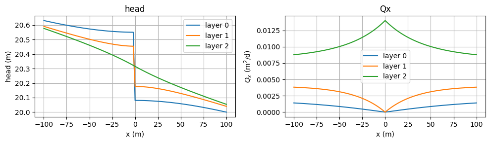
Impermeable wall#
Flow from left to right in three-layer aquifer with impermeable wall in bottom 2 layers
# need ModelMaq here since Uflow requires a confined background aquifer
ml = tfs.ModelMaq(kaq=[1, 2, 4], z=[5, 4, 3, 2, 1, 0], c=[5000, 1000])
uf = tfs.Uflow(ml, 0.002, 0)
rf = tfs.Constant(ml, 100, 0, 20)
ld1 = tfs.ImpermeableWall1D(ml, xld=0, layers=[0, 1])

ml.solve()
Number of elements, Number of equations: 3 , 3
.
.
.

solution complete
x = np.linspace(-100, 100, 101)
h = ml.headalongline(x, np.zeros_like(x))
Qx, _ = ml.disvecalongline(x, np.zeros_like(x))

plt.figure(figsize=(10, 3))
plt.subplot(121)
plt.title("head")
plt.plot(x, h[0], label="layer 0")
plt.plot(x, h[1], label="layer 1")
plt.plot(x, h[2], label="layer 2")
plt.xlabel("x (m)")
plt.ylabel("head (m)")
plt.legend(loc="best")
plt.grid()
plt.subplot(122)
plt.title("Qx")
plt.plot(x, Qx[0], label="layer 0")
plt.plot(x, Qx[1], label="layer 1")
plt.plot(x, Qx[2], label="layer 2")
plt.xlabel("x (m)")
plt.ylabel("$Q_x$ (m$^2$/d)")
plt.legend(loc="best")
plt.grid()
ax = ml.plots.vcontoursf1D(
    x1=-200, x2=200, nx=100, levels=20, color="C0", figsize=(10, 3), horizontal_axis="x"
)
ld1.plot(ax);  # plot wall
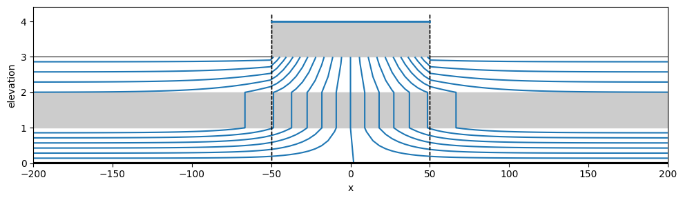
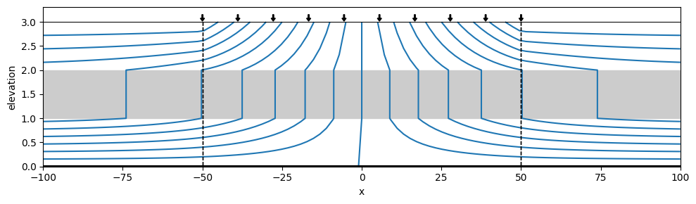
Infiltration#
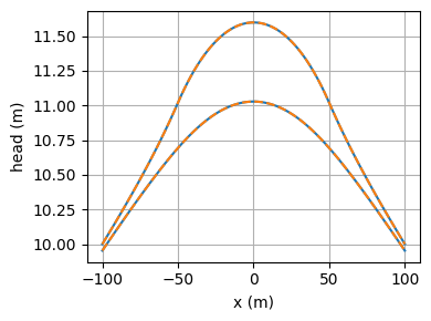
Comparing solution with Xsection inhomogeneities to XsectionAreaSink solution.
ml = tfs.ModelXsection(naq=2)
tfs.XsectionMaq(
    ml,
    x1=-np.inf,
    x2=-50,
    kaq=[1, 2],
    z=[3, 2, 1, 0],
    c=[1000],
    npor=0.3,
    topboundary="conf",
)
tfs.XsectionMaq(
    ml,
    x1=-50,
    x2=50,
    kaq=[1, 2],
    z=[3, 2, 1, 0],
    c=[1000],
    npor=0.3,
    topboundary="conf",
    N=0.001,
)
tfs.XsectionMaq(
    ml,
    x1=50,
    x2=np.inf,
    kaq=[1, 2],
    z=[3, 2, 1, 0],
    c=[1000],
    npor=0.3,
    topboundary="conf",
)
tfs.Constant(ml, -100, 0, 10)
tfs.Constant(ml, 100, 0, 10)
ml.solve()

ml.plots.vcontoursf1D(x1=-100, x2=100, nx=100, levels=20, color="C0", figsize=(10, 3));
Number of elements, Number of equations: 7 , 10
.
.
.
.
.
.
.

solution complete
ml2 = tfs.ModelMaq(kaq=[1, 2], z=[3, 2, 1, 0], c=[1000], topboundary="conf")
tfs.XsectionAreaSink(ml2, -50, 50, 0.001)
tfs.Constant(ml2, -100, 0, 10)
ml2.solve()
ml2.plots.vcontoursf1D(
    x1=-100, x2=100, nx=100, levels=20, color="C0", figsize=(10, 3), horizontal_axis="x"
);
Number of elements, Number of equations: 2 , 1
.
.

solution complete
/tmp/ipykernel_1214/2937150034.py:2: DeprecationWarning: XsectionAreaSink is only for testing purposes. It is recommended to add infiltration through XsectionMaq or Xsection3D and specifying 'N'.
  tfs.XsectionAreaSink(ml2, -50, 50, 0.001)
x = np.linspace(-100, 100, 100)
plt.plot(x, ml.headalongline(x, 0)[0], "C0")
plt.plot(x, ml.headalongline(x, 0)[1], "C0")
plt.plot(x, ml2.headalongline(x, 0)[0], "--C1")
plt.plot(x, ml2.headalongline(x, 0)[1], "--C1")
plt.xlabel("x (m)")
plt.ylabel("head (m)")
plt.grid()
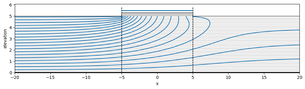
ml = tfs.ModelXsection(naq=50)
tfs.Xsection3D(ml, x1=-np.inf, x2=-5, kaq=1, z=np.arange(5, -0.1, -0.1), kzoverkh=0.1)
tfs.Xsection3D(
    ml,
    x1=-5,
    x2=5,
    kaq=1,
    z=np.arange(5, -0.1, -0.1),
    kzoverkh=0.1,
    topboundary="semi",
    hstar=5.5,
    topres=3,
    topthick=0.3,
)
tfs.Xsection3D(ml, x1=5, x2=np.inf, kaq=1, z=np.arange(5, -0.1, -0.1), kzoverkh=0.1)
rf1 = tfs.Constant(ml, -100, 0, 5.7)
rf2 = tfs.Constant(ml, 100, 0, 5.47)

ml.solve()

ml.plots.vcontoursf1D(x1=-20, x2=20, nx=100, levels=20, color="C0", figsize=(10, 3));
Number of elements, Number of equations: 7 , 202
.
.
.
.
.
.
.

solution complete
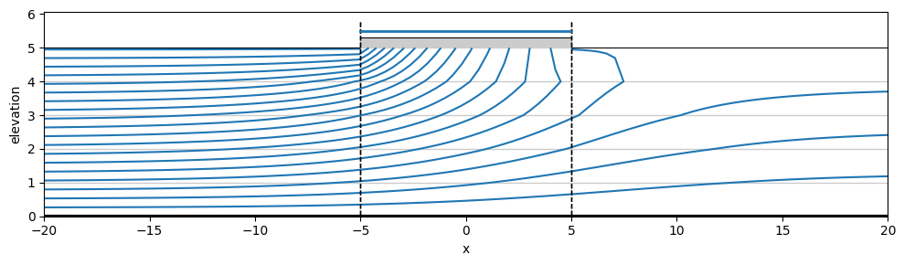
ml = tfs.ModelXsection(naq=5)
tfs.Xsection3D(ml, x1=-np.inf, x2=-5, kaq=1, z=np.arange(5, -0.1, -1), kzoverkh=0.1)
tfs.Xsection3D(
    ml,
    x1=-5,
    x2=5,
    kaq=1,
    z=np.arange(5, -0.1, -1),
    kzoverkh=0.1,
    topboundary="semi",
    hstar=5.5,
    topres=3,
    topthick=0.3,
)
tfs.Xsection3D(ml, x1=5, x2=np.inf, kaq=1, z=np.arange(5, -0.1, -1), kzoverkh=0.1)
rf1 = tfs.Constant(ml, -100, 0, 5.7)
rf2 = tfs.Constant(ml, 100, 0, 5.47)

ml.solve()

ml.plots.vcontoursf1D(x1=-20, x2=20, nx=100, levels=20, color="C0", figsize=(10, 3));
Number of elements, Number of equations: 7 , 22
.
.
.
.
.
.
.

solution complete
ml = tfs.ModelXsection(naq=2)
tfs.XsectionMaq(
    ml,
    x1=-np.inf,
    x2=-50,
    kaq=[1, 2],
    z=[4, 3, 2, 1, 0],
    c=[1000, 1000],
    npor=0.3,
    topboundary="semi",
    hstar=15,
)
tfs.XsectionMaq(
    ml,
    x1=-50,
    x2=50,
    kaq=[1, 2],
    z=[4, 3, 2, 1, 0],
    c=[1000, 1000],
    npor=0.3,
    topboundary="semi",
    hstar=13,
)
tfs.XsectionMaq(
    ml,
    x1=50,
    x2=np.inf,
    kaq=[1, 2],
    z=[4, 3, 2, 1, 0],
    c=[1000, 1000],
    npor=0.3,
    topboundary="semi",
    hstar=11,
)
ml.solve()
Number of elements, Number of equations: 7 , 8
.
.
.
.
.
.
.

solution complete
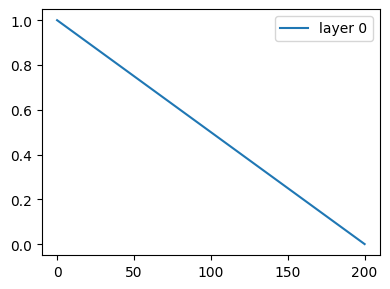
from timflow.steady.linesink1d import FluxDiffLineSink1D, HeadDiffLineSink1D
ml = tfs.ModelMaq(kaq=[10], z=[0, -10], topboundary="conf")
ls = tfs.River1D(ml, xls=0, hls=1, wh="H", layers=0)
ls = tfs.River1D(ml, xls=200, hls=0, wh="H", layers=0)
hd = HeadDiffLineSink1D(ml, xls=100)
fd = FluxDiffLineSink1D(ml, xls=100)
ml.solve()

x = np.linspace(0, 200, 101)
h = ml.headalongline(x, np.zeros_like(x))
plt.plot(x, h[0], label="layer 0")
# plt.plot(x, h[1], label="layer 1")
plt.legend(loc="best");
Number of elements, Number of equations: 2 , 2
.
.

solution complete