Test line-sink discharge#
import matplotlib.pyplot as plt
import numpy as np

import timflow.steady as tfs

plt.rcParams["figure.figsize"] = (4, 3)
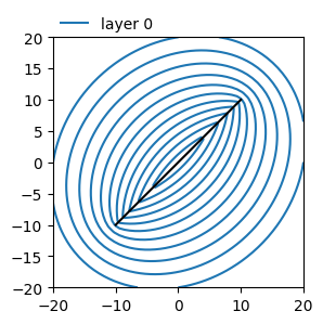
Comparison of one line-sink with uniform strength to a row of wells with constant strength.#
ml1 = tfs.ModelMaq(kaq=20)
rf1 = tfs.Constant(ml1, xr=0, yr=20, hr=30)
ls1 = tfs.LineSinkBase(ml1, x1=-10, y1=-10, x2=10, y2=10, Qls=1000)
ml1.solve()
Number of elements, Number of equations: 2 , 1
.
.

solution complete
print("head at center of line-sink:", ml1.head(ls1.xc[0], ls1.yc[0]))
print("discharge of line-sink:", ls1.discharge())
head at center of line-sink: [19.19104524]
discharge of line-sink: [1000.]
ml2 = tfs.ModelMaq(kaq=20)
rf2 = tfs.Constant(ml2, xr=0, yr=20, hr=30)
N = 20
d = 20 / N
xw = np.arange(-10 + d / 2, 10, d)
yw = np.arange(-10 + d / 2, 10, d)
for i in range(N):
    tfs.Well(ml2, xw[i], yw[i], Qw=1000 / N)
ml2.solve(silent=True)
ml1.plots.contour(
    [-20, 20, -20, 20], 50, [0], np.arange(20, 31, 1), color="C0", labels=False
)
ml2.plots.contour(
    [-20, 20, -20, 20],
    50,
    [0],
    np.arange(20, 31, 1),
    color="C1",
    labels=False,
    newfig=False,
)
/home/docs/checkouts/readthedocs.org/user_builds/timflow/envs/27/lib/python3.13/site-packages/timflow/steady/plots.py:119: UserWarning: The following kwargs were not used by contour: 'newfig'
  cs = ax.contour(xg, yg, h[i], levels, colors=c[i], **kwargs)
<Axes: >
Head line-sink of higher order with control point on the line-sink#
ml1 = tfs.ModelMaq(kaq=[20, 10], z=[20, 12, 10, 0], c=[100])
rf1 = tfs.Constant(ml1, xr=0, yr=20, hr=30)
ls1 = tfs.River(ml1, -10, 0, 10, 0, 20, order=7, layers=0)  # set control point at y=0.5
ml1.solve()

for icp in range(ls1.ncp):
    print("icp, head inside: ", icp, ls1.headinside(icp))
Number of elements, Number of equations: 2 , 9
.
.

solution complete
icp, head inside:  0 [20.]
icp, head inside:  1 [20.]
icp, head inside:  2 [20.]
icp, head inside:  3 [20.]
icp, head inside:  4 [20.]
icp, head inside:  5 [20.]
icp, head inside:  6 [20.]
icp, head inside:  7 [20.]
Head line-sink of higher order with control point \(\Delta y\) off line-sink#
Useful when line-sink is used to simulate horizontal well with finite radius or ditch with finite width. Note that this means that the head inside this distance \(\Delta y\) is essentially meaningless (but a value is returned)
ml1 = tfs.ModelMaq(kaq=[20, 10], z=[20, 12, 10, 0], c=[100])
rf1 = tfs.Constant(ml1, xr=0, yr=20, hr=30)
ls1 = tfs.River(
    ml1, -10, 0, 10, 0, 20, order=7, layers=0, dely=0.5
)  # set control point at 0.5 from line-sink
ml1.solve()

for icp in range(ls1.ncp):
    print("icp, head inside: ", icp, ls1.headinside(icp))
Number of elements, Number of equations: 2 , 9
.
.

solution complete
icp, head inside:  0 [20.]
icp, head inside:  1 [20.]
icp, head inside:  2 [20.]
icp, head inside:  3 [20.]
icp, head inside:  4 [20.]
icp, head inside:  5 [20.]
icp, head inside:  6 [20.]
icp, head inside:  7 [20.]
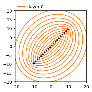
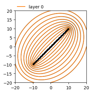
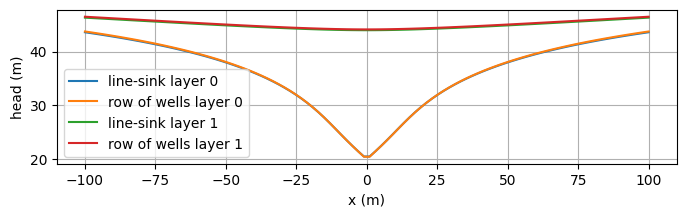
Comparison of head line-sink with row of well with specified head.#
ml1 = tfs.ModelMaq(kaq=[20, 10], z=[20, 12, 10, 0], c=[100])
rf1 = tfs.Constant(ml1, xr=0, yr=20, hr=30)
ls1 = tfs.River(ml1, -10, -10, 10, 10, 20, order=7, layers=0)
ml1.solve()
Number of elements, Number of equations: 2 , 9
.
.

solution complete
ml2 = tfs.ModelMaq(kaq=[20, 10], z=[20, 12, 10, 0], c=[100])
rf2 = tfs.Constant(ml2, xr=0, yr=20, hr=30)
N = 50
d = 20 / N
xw = np.arange(-10 + d / 2, 10, d)
yw = np.arange(-10 + d / 2, 10, d)
for i in range(N):
    tfs.HeadWell(ml2, xw[i], yw[i], 20, layers=0)
ml2.solve(silent=True)
Qwell = 0
for i in range(N):
    Qwell += ml2.elementlist[i + 1].discharge()
print("discharge of line-sink:", ls1.discharge())
print("discharge of wells:", Qwell)
discharge of line-sink: [9430.33419678    0.        ]
discharge of wells: [9527.67795022    0.        ]
ax = ml1.plots.contour(
    [-20, 20, -20, 20], 50, [0], np.arange(20, 31, 1), color="C0", labels=False
)
ml2.plots.contour(
    [-20, 20, -20, 20],
    50,
    [0],
    np.arange(20, 31, 1),
    color="C1",
    labels=False,
    ax=ax,
)
<Axes: >
x = np.linspace(-100, 100, 100)
h1 = ml1.headalongline(x, 0)
h2 = ml2.headalongline(x, 0)
plt.figure(figsize=(8, 2))
for ilay in range(2):
    plt.plot(x, h1[ilay], label=f"line-sink layer {ilay}")
    plt.plot(x, h2[ilay], label=f"row of wells layer {ilay}")
plt.xlabel("x (m)")
plt.ylabel("head (m)")
plt.legend()
plt.grid()
Higher-order head line-sink with resistance#
ml = tfs.ModelMaq(kaq=3, z=[10, 0])
ls1 = tfs.River(ml, -10, 0, 10, 0, hls=2, wh=1, res=0.2, order=2)
rf = tfs.Constant(ml, 0, 20, 4)
ml.solve()
Number of elements, Number of equations: 2 , 4
.
.

solution complete
print("inflow at each control-point")
for i in range(3):
    print(
        i,
        (ml.head(ls1.xc[i], ls1.yc[i]) - ls1.hc[i]) * ls1.wh / ls1.res,
        np.sum(ls1.strengthinf[i] * ls1.parameters[:, 0]),
    )
inflow at each control-point
0 [5.71224596] 5.7122459642992895
1 [5.08470557] 5.084705571057445
2 [5.71224596] 5.712245964299295
print("head inside at each control point")
for i in range(3):
    print("icp, head: ", i, ls1.headinside(i))
head inside at each control point
icp, head:  0 [2.]
icp, head:  1 [2.]
icp, head:  2 [2.]
Higher order head line-sink with resistance in one layer of multiple layers system#
ml = tfs.ModelMaq(kaq=[1, 2], z=[20, 10, 10, 0], c=[1000])
lslayer = 0
order = 2
ls1 = tfs.River(ml, -10, 0, 10, 0, hls=-2, order=order, wh=1, res=2, layers=[lslayer])
rf = tfs.Constant(ml, 0, 20, 2)
ml.solve()

for icp in range(ls1.ncp):
    print("icp, head inside: ", icp, ls1.headinside(icp))
Number of elements, Number of equations: 2 , 4
.
.

solution complete
icp, head inside:  0 [-2.]
icp, head inside:  1 [-2.]
icp, head inside:  2 [-2.]
ml = tfs.ModelMaq(kaq=[1, 2], z=[20, 12, 10, 0], c=[1000])
order = 2
ls1 = tfs.River(ml, -10, 0, 10, 0, hls=-2, order=order, wh=1, res=2, layers=[0, 1])
rf = tfs.Constant(ml, 0, 2000, 2)
ml.solve()

print("inflow at each control-point")
for i in range(order + 1):
    print(
        i,
        (ml.head(ls1.xc[i], ls1.yc[i]) - ls1.hc[i])[lslayer] * ls1.wh / ls1.res,
        np.sum(ls1.strengthinf[i] * ls1.parameters[:, 0]),
    )
print("head inside at each control point")
for icp in range(ls1.ncp):
    print("icp, head inside: ", icp, ls1.headinside(icp))
Number of elements, Number of equations: 2 , 7
.
.

solution complete
inflow at each control-point
0 1.0174441975895396 1.0174441975895407
1 0.9680577364621308 1.2960716857825254
2 1.0174441975895396 0.9680577364621321
head inside at each control point
icp, head inside:  0 [-2. -2.]
icp, head inside:  1 [-2. -2.]
icp, head inside:  2 [-2. -2.]
Specifying heads along line-sinks#
Give one value that is applied at all control points
ml1 = tfs.ModelMaq(kaq=[20, 10], z=[20, 12, 10, 0], c=[100])
rf1 = tfs.Constant(ml1, xr=0, yr=20, hr=30)
ls1 = tfs.River(ml1, -10, 0, 10, 0, hls=20, order=2, layers=[0])
ml1.solve()
print(ml1.headalongline(ls1.xc, ls1.yc))
Number of elements, Number of equations: 2 , 4
.
.

solution complete
[[20.         20.         20.        ]
 [39.70172813 39.68117849 39.70172813]]
Give order + 1 values, which is applied at the order + 1 control points. This may not be so useful, as the user needs to know where those control points are.
ml1 = tfs.ModelMaq(kaq=[20, 10], z=[20, 12, 10, 0], c=[100])
rf1 = tfs.Constant(ml1, xr=0, yr=20, hr=30)
ls1 = tfs.River(ml1, -10, 0, 10, 0, hls=[20, 19, 18], order=2, layers=[0])
ml1.solve()
print(ml1.headalongline(ls1.xc, ls1.yc))
Number of elements, Number of equations: 2 , 4
.
.

solution complete
[[20.         19.         18.        ]
 [40.67762937 40.64929634 40.66617251]]
Give two values, the head at the beginning and end of the line-sink. Linear interpolation in between.
ml1 = tfs.ModelMaq(kaq=[20, 10], z=[20, 12, 10, 0], c=[100])
rf1 = tfs.Constant(ml1, xr=0, yr=20, hr=30)
ls1 = tfs.River(ml1, -10, 0, 10, 0, hls=[19, 20], order=2, layers=[0])
ml1.solve()
print(ml1.headalongline(ls1.xc, ls1.yc))
Number of elements, Number of equations: 2 , 4
.
.

solution complete
[[19.14644661 19.5        19.85355339]
 [40.18478923 40.16523741 40.18883984]]
Ditch#
Specify total discharge of ditch. Uniform head inside ditch is computed.
Single ditch in one layer of two-aquifer system.
ml1 = tfs.ModelMaq(kaq=[20, 10], z=[20, 12, 10, 0], c=[100])
rf1 = tfs.Constant(ml1, xr=0, yr=20, hr=30)
ls1 = tfs.Ditch(ml1, -10, -10, 10, 10, Qls=1000, order=2, layers=[0])
ml1.solve()
for icp in range(ls1.ncp):
    print("icp, head inside: ", icp, ls1.headinside(icp))
Number of elements, Number of equations: 2 , 4
.
.

solution complete
icp, head inside:  0 [28.88125554]
icp, head inside:  1 [28.88125554]
icp, head inside:  2 [28.88125554]
Single ditch with resistance, in both layers of two-aquifer system.
ml1 = tfs.ModelMaq(kaq=[20, 10], z=[20, 12, 10, 0], c=[100])
rf1 = tfs.Constant(ml1, xr=0, yr=20, hr=30)
ls1 = tfs.Ditch(ml1, -10, -10, 10, 10, Qls=1000, order=2, res=0.1, layers=[0, 1])
ml1.solve()
for icp in range(ls1.ncp):
    print("icp, head inside: ", icp, ls1.headinside(icp))
print("discharge: ", ls1.discharge())
print("total discharge: ", np.sum(ls1.discharge()))
Number of elements, Number of equations: 2 , 7
.
.

solution complete
icp, head inside:  0 [27.3827848 27.3827848]
icp, head inside:  1 [27.3827848 27.3827848]
icp, head inside:  2 [27.3827848 27.3827848]
discharge:  [556.70589094 443.29410906]
total discharge:  1000.0
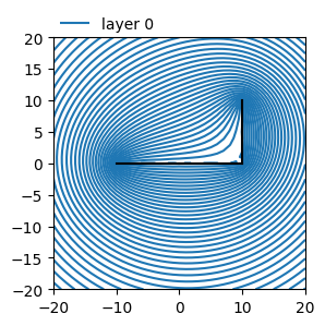
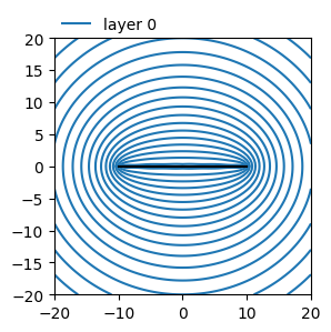
Head line-sink string#
ml1 = tfs.ModelMaq(kaq=[20, 10], z=[20, 12, 10, 0], c=[100])
rf1 = tfs.Constant(ml1, xr=0, yr=20, hr=30)
ls1 = tfs.RiverString(
    ml1, xy=[(-10, 0), (0, 0), (10, 0), (10, 10)], hls=20, order=5, layers=[0]
)
ml1.solve()
ml1.plots.contour([-20, 20, -20, 20], 41, [0], 40, labels=False)
for ils in range(ls1.nls):
    print("line-sink, head inside: ", ils, ls1.lslist[ils].headinside())
Number of elements, Number of equations: 2 , 19
.
.

solution complete
line-sink, head inside:  0 [20.]
line-sink, head inside:  1 [20.]
line-sink, head inside:  2 [20.]
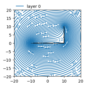
Head line-sink string with linearly varying head.
# linearly varying head along line-sink
ml1 = tfs.ModelMaq(kaq=[20, 10], z=[20, 12, 10, 0], c=[100])
rf1 = tfs.Constant(ml1, xr=0, yr=20, hr=30)
ls1 = tfs.RiverString(
    ml1, xy=[(-10, 0), (0, 0), (10, 0), (10, 10)], hls=[20, 22], order=5, layers=[0]
)
ml1.solve()
ml1.plots.contour([-20, 20, -20, 20], 41, [0], 40)
for ils in range(ls1.nls):
    print("line-sink, spec head, head inside: ", ils, ls1.lslist[ils].hc)
    for icp in range(ls1.lslist[ils].ncp):
        print("icp, head ", ls1.lslist[ils].headinside(icp))
Number of elements, Number of equations: 2 , 19
.
.

solution complete
line-sink, spec head, head inside:  0 [20.03301038 20.1255034  20.25915969 20.40750698 20.54116327 20.63365629]
icp, head  [20.03301038]
icp, head  [20.1255034]
icp, head  [20.25915969]
icp, head  [20.40750698]
icp, head  [20.54116327]
icp, head  [20.63365629]
line-sink, spec head, head inside:  1 [20.69967704 20.79217007 20.92582636 21.07417364 21.20782993 21.30032296]
icp, head  [20.69967704]
icp, head  [20.79217007]
icp, head  [20.92582636]
icp, head  [21.07417364]
icp, head  [21.20782993]
icp, head  [21.30032296]
line-sink, spec head, head inside:  2 [21.36634371 21.45883673 21.59249302 21.74084031 21.8744966  21.96698962]
icp, head  [21.36634371]
icp, head  [21.45883673]
icp, head  [21.59249302]
icp, head  [21.74084031]
icp, head  [21.8744966]
icp, head  [21.96698962]
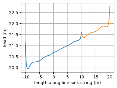
xls1 = np.linspace(-10, 10, 50)
yls1 = np.linspace(0, 0, 50)
hls1 = ml1.headalongline(xls1, yls1)
plt.figure()
plt.plot(xls1, hls1[0])
xls2 = np.linspace(10, 10, 50)
yls2 = np.linspace(0, 10, 50)
hls2 = ml1.headalongline(xls2, yls2)
plt.plot(10 + yls2, hls2[0])
plt.xlabel("length along line-sink string (m)")
plt.ylabel("head (m)")
plt.grid()
Head line-sink string with resistance.
ml1 = tfs.ModelMaq(kaq=[20, 10], z=[20, 12, 10, 0], c=[100])
rf1 = tfs.Constant(ml1, xr=0, yr=200, hr=2)
ls1 = tfs.RiverString(
    ml1,
    xy=[(-10, 0), (0, 0), (10, 0), (10, 10)],
    hls=1,
    res=2,
    wh=5,
    order=5,
    layers=[0],
)
ml1.solve()
Number of elements, Number of equations: 2 , 19
.
.

solution complete
for ils in range(ls1.nls):
    for icp in range(ls1.lslist[ils].ncp):
        print("ils, icp, head inside:", ils, icp, ls1.lslist[ils].headinside(icp))
ils, icp, head inside: 0 0 [1.]
ils, icp, head inside: 0 1 [1.]
ils, icp, head inside: 0 2 [1.]
ils, icp, head inside: 0 3 [1.]
ils, icp, head inside: 0 4 [1.]
ils, icp, head inside: 0 5 [1.]
ils, icp, head inside: 1 0 [1.]
ils, icp, head inside: 1 1 [1.]
ils, icp, head inside: 1 2 [1.]
ils, icp, head inside: 1 3 [1.]
ils, icp, head inside: 1 4 [1.]
ils, icp, head inside: 1 5 [1.]
ils, icp, head inside: 2 0 [1.]
ils, icp, head inside: 2 1 [1.]
ils, icp, head inside: 2 2 [1.]
ils, icp, head inside: 2 3 [1.]
ils, icp, head inside: 2 4 [1.]
ils, icp, head inside: 2 5 [1.]
Calculate total discharge and per linesink (using two different methods), check they are all equal.
Qtot = ls1.discharge()
Qls_sum = np.sum(ls1.discharge_per_linesink(), axis=1)
Qper_linesink_sum = np.sum([e.discharge() for e in ls1.lslist], axis=0)


assert np.allclose(Qtot, Qls_sum)
assert np.allclose(Qtot, Qper_linesink_sum)
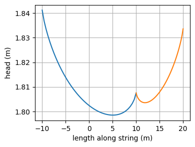
# plot head in aquifer along line-sink string
# (note there is a resistance, so this is not constant)
xls1 = np.linspace(-10, 10, 50)
yls1 = np.linspace(0, 0, 50)
hls1 = ml1.headalongline(xls1, yls1)
plt.figure()
plt.plot(xls1, hls1[0])
xls2 = np.linspace(10, 10, 50)
yls2 = np.linspace(0, 10, 50)
hls2 = ml1.headalongline(xls2, yls2)
plt.plot(10 + yls2, hls2[0])
plt.xlabel("length along string (m)")
plt.ylabel("head (m)")
plt.grid()
Ditch string#
Ditch string without resistance, screened in one layer.
ml1 = tfs.ModelMaq(kaq=[20, 10], z=[20, 12, 10, 0], c=[100])
rf1 = tfs.Constant(ml1, xr=0, yr=20, hr=1)
ls1 = tfs.DitchString(
    ml1, xy=[(-10, 0), (0, 0), (10, 0)], Qls=100, res=0, order=5, layers=[0]
)

ml1.solve()
print("discharge:", ls1.discharge())

for ils in range(ls1.nls):
    for icp in range(ls1.lslist[ils].ncp):
        print("ils, icp, head inside:", ils, icp, ls1.lslist[ils].headinside(icp))
Number of elements, Number of equations: 2 , 13
.
.

solution complete
discharge: [100.   0.]
ils, icp, head inside: 0 0 [0.85647874]
ils, icp, head inside: 0 1 [0.85647874]
ils, icp, head inside: 0 2 [0.85647874]
ils, icp, head inside: 0 3 [0.85647874]
ils, icp, head inside: 0 4 [0.85647874]
ils, icp, head inside: 0 5 [0.85647874]
ils, icp, head inside: 1 0 [0.85647874]
ils, icp, head inside: 1 1 [0.85647874]
ils, icp, head inside: 1 2 [0.85647874]
ils, icp, head inside: 1 3 [0.85647874]
ils, icp, head inside: 1 4 [0.85647874]
ils, icp, head inside: 1 5 [0.85647874]
ml1.plots.contour([-20, 20, -20, 20], 81, [0], 20, labels=False)
<Axes: >
Ditch in multiple layers with resistance.
ml1 = tfs.ModelMaq(kaq=[20, 10], z=[20, 12, 10, 0], c=[100])
rf1 = tfs.Constant(ml1, xr=0, yr=20, hr=1)
ls1 = tfs.DitchString(
    ml1, xy=[(-10, 0), (0, 0), (10, 0)], Qls=100, res=0.2, order=5, layers=[0, 1]
)

ml1.solve()
print("discharge:", ls1.discharge())

for ils in range(ls1.nls):
    for icp in range(ls1.lslist[ils].ncp):
        print("ils, icp, head inside:", ils, icp, ls1.lslist[ils].headinside(icp))
Number of elements, Number of equations: 2 , 13
.
.

solution complete
discharge: [52.21451036 47.78548964]
ils, icp, head inside: 0 0 [-0.16022727]
ils, icp, head inside: 0 1 [-0.16022727]
ils, icp, head inside: 0 2 [-0.16022727]
ils, icp, head inside: 0 3 [-0.16022727]
ils, icp, head inside: 0 4 [-0.16022727]
ils, icp, head inside: 0 5 [-0.16022727]
ils, icp, head inside: 1 0 [-0.16022727]
ils, icp, head inside: 1 1 [-0.16022727]
ils, icp, head inside: 1 2 [-0.16022727]
ils, icp, head inside: 1 3 [-0.16022727]
ils, icp, head inside: 1 4 [-0.16022727]
ils, icp, head inside: 1 5 [-0.16022727]
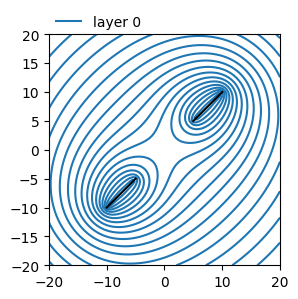
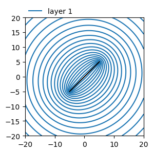
Ditch in different layers#
ml1 = tfs.ModelMaq(kaq=[20, 10], z=[20, 12, 10, 0], c=[100])
rf1 = tfs.Constant(ml1, xr=0, yr=20, hr=1)
ls1 = tfs.DitchString(
    ml1,
    xy=[(-10, -10), (-5, -5), (5, 5), (10, 10)],
    Qls=100,
    wh=2,
    res=0,
    order=5,
    layers=[0, 1, 0],
)
ml1.solve()

for ils in range(ls1.nls):
    for icp in range(ls1.lslist[ils].ncp):
        print("ils, icp, head inside:", ils, icp, ls1.lslist[ils].headinside(icp))
Number of elements, Number of equations: 2 , 19
.
.

solution complete
ils, icp, head inside: 0 0 [0.91994398]
ils, icp, head inside: 0 1 [0.91994398]
ils, icp, head inside: 0 2 [0.91994398]
ils, icp, head inside: 0 3 [0.91994398]
ils, icp, head inside: 0 4 [0.91994398]
ils, icp, head inside: 0 5 [0.91994398]
ils, icp, head inside: 1 0 [0.91994398]
ils, icp, head inside: 1 1 [0.91994398]
ils, icp, head inside: 1 2 [0.91994398]
ils, icp, head inside: 1 3 [0.91994398]
ils, icp, head inside: 1 4 [0.91994398]
ils, icp, head inside: 1 5 [0.91994398]
ils, icp, head inside: 2 0 [0.91994398]
ils, icp, head inside: 2 1 [0.91994398]
ils, icp, head inside: 2 2 [0.91994398]
ils, icp, head inside: 2 3 [0.91994398]
ils, icp, head inside: 2 4 [0.91994398]
ils, icp, head inside: 2 5 [0.91994398]
ml1.plots.contour([-20, 20, -20, 20], 81, layers=[0], levels=20, labels=False)
<Axes: >
ml1.plots.contour([-20, 20, -20, 20], 81, layers=[1], levels=20, labels=False)
<Axes: >
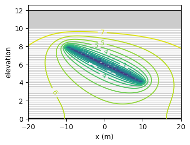
Angle well#
ml = tfs.Model3D(
    kaq=1,
    z=np.arange(10, -0.1, -0.2),
    kzoverkh=0.1,
    topboundary="semi",
    topres=0,
    topthick=2,
    hstar=7,
)
xy = list(zip(np.linspace(-10, 10, 21), np.zeros(21), strict=False))
ls1 = tfs.DitchString(
    ml, xy=xy, Qls=100, wh=2, res=5, order=2, layers=np.arange(10, 30, 1)
)
ml.solve()
Number of elements, Number of equations: 2 , 60
.
.

solution complete
ml.plots.vcontour(win=[-20, 20, 0, 0], n=100, levels=20, layout=True, horizontal_axis="x")
plt.xlabel("x (m)");