Tutorial 1: Well in a Multi-Aquifer System

Uniform flow to a well in a multi-aquifer system

In this notebook, we will simulate steady flow to an extraction well in the middle aquifer of a three-aquifer system. Aquifer properties are given in the table shown below. The well is located at \((x,y)=(0,0)\), the discharge is \(Q=10,000\) m\(^3\)/d and the radius is 0.2 m. There is a uniform flow from West to East with a gradient of 0.002. The head is fixed to 20 m at a distance of 10,000 m downstream of the well.

Aquifer properties

Layer	\(k\) (m/d)	\(z_b\) (m)	\(z_t\)	\(c\) (days)
Aquifer 0	10	-20	0	-
Leaky Layer 1	-	-40	-20	4000
Aquifer 1	20	-80	-40	-
Leaky Layer 2	-	-90	-80	10000
Aquifer 2	5	-140	-90	-

We start the model by importing the regular packages and timflow.steady.

import numpy as np

import timflow.steady as tfs

We create a multi-aquifer model with the ModelMaq class. We specify the hydraulic conductivitity for each aquifer (kaq), followed by a vector z with the top and bottom of each aquifer from the top down (i.e., 6 values, as there are 3 aquifers). The model instance is stored in the variable ml. Next, three elements are added to the model: a well (Well), a reference point with a fixed head (Constant), and uniform flow (Uflow). The well is screened in the middle aquifer layer (which is number 1). Since it is screened in only 1 layer, it suffices to provide one value for the keyword layers. The well is stored in the variable w for later use. The reference point is added by specifying the location, the head, and the layer. Note that only one reference point can be added to the model and in only one layer (hence, the keyword is layer and not layers).

ml = tfs.ModelMaq(
    kaq=[10, 20, 5],  # hydraulic conductivity, m/d
    z=[0, -20, -40, -80, -90, -140],  # tops and bottoms of aquifers, m
    c=[4000, 10000],  # resistance of leaky layers, d
    npor=0.3,  # porosity of the aquifers, one value so the same for all aquifers, -
)
w = tfs.Well(
    model=ml,  # model to which element is added
    xw=0,  # x-location of well, m
    yw=0,  # y-location of well, m
    Qw=10_000,  # discharge of well, positive for extraction, m^3/d
    rw=0.2,  # well radius, m
    layers=1,  # layer numbere where well is screened (may also be a list)
    label="well 1",
)
tfs.Constant(
    model=ml,  # model to which element is added
    xr=10_000,  # x-location of fixed head, m
    yr=0,  # y-location of fixed head, m
    hr=20,  # fixed head, m
    layer=0,  # layer number where head is fixed
)
tfs.Uflow(
    model=ml,  # model to which element is added
    slope=0.002,  # head drop / distance in direction of flow
    angle=0,  # direction of uniform flow, straight East is zero degrees
)
ml.solve()  # solve the model

Number of elements, Number of equations: 3 , 1
.
.
.

solution complete

w.nunknowns

0

The transmissivity of each aquifer is computed and stored by timflow. Each timflow model stores all aquifer properties as aq. The transmissivities are stored in the variable T

ml.aq.T

array([200., 800., 250.])

This means that the transmissivity of the middle aquifer is 800 m\(^2\)/d (as is indeed the product of the hydraulic conductivity and thickness of aquifer layer 1, see the values in the table).

A confined aquifer system with three aquifer layers and two leaky layers has two leakage factors. The heads in all three aquifers are approximately equal at a distance of three times the largest leakage factor away from the well. The leakage factors are computed by timflow and may be obtained as follows:

print("leakage factors of model (m)")
print(ml.aq.lab)

leakage factors of model (m)
[   0.         1430.58042146  790.84743012]

Note that timflow actually returns three leakage factors (as the system consists of three aquifers), but since the top of the aquifer system is impermeable, the first leakage factor is equal to 0 (it will be a non-zero value for a semi-confined system, where the top aquifer is covered by a leaky layer with a fixed head above it).

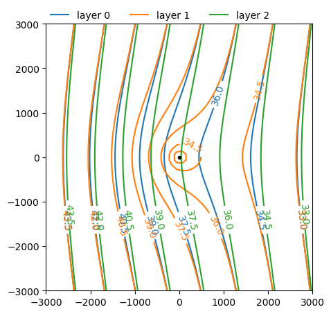
One contour plot of the heads in all three aquifers is created. Contours are drawn inside a window with lower-left hand corner \((x,y)=(−3000,−3000)\) and upper right-hand corner \((x,y)=(3000,3000)\). Notice that the heads in the three aquifers are almost equal at three times the largest leakage factor.

ml.plots.contour(
    win=[-3000, 3000, -3000, 3000],  # window to contour [xmin, xmax, ymin, ymax]
    ngr=50,  # number of points where to compute the head
    layers=[0, 1, 2],  # layers to contour
    levels=10,  # draw 10 contours in each layer
    labels=True,  # add labels along the contours
    decimals=1,  # print labels with 1 decimal place
    legend=True,  # add a legend
    figsize=(5, 5),  # specify a figure size of 5 by 5 inches
);

The head in the well is computed as before. Note that the drawdown is quite large, as the head at the well is 40 m in absence of the well.

print(f"The head at the well is: {w.headinside()} m")

The head at the well is: [20.06196743] m

The head at the well may also be computed with the ml.head function, which returns the head at the well in all three layers. (The careful reader may note that the head in layer 1 is slightly different than the value obtained with w.headinside, because the head is computed slightly different, but the difference is less than 1 mm.)

ml.head(0, 0)

array([36.67647333, 20.06236743, 37.57926023])

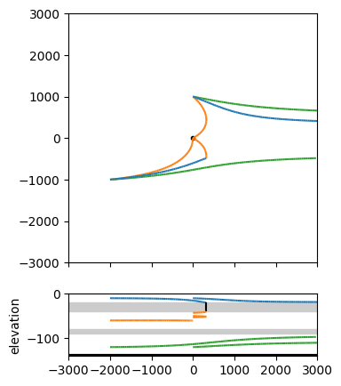
Finally, six pathlines are computed and plotted in both a plan view and a cross-section. Three pathlines are started from from \((x,y)=(-2000,-1000)\), but at three different levels \(z=-120\), \(z=-60\), and \(z=-10\) (i.e., one from each aquifer). The other three pathlines are started from the same elevations, but from \((x,y)=(0, 1000)\). A plot of the aquifer must be created before pathlines can be visualized. In the code cell below, the plot is created with the ml.plot function, which only plots the elements to the screen (in this case only the well, as there are no elements to visualize). In addition, the orientation is set to both, which means that both a plan view and a vertical cross-section are plotted. Note that the pathlines are automatically colored: they are blue (C0) in aquifer 0, orange (C1) in aquifer 1 and green (C2) in aquifer 2. Note that the pathline that starts in the top aquifer at \((-2000, -1000)\) leaks to the middle aquifer (when it changes from blue to orange) and ends at the well.

win = [-3000, 3000, -3000, 3000]  # window that is plotted [xmin, xmax, ymin, ymax]
axes = ml.plots.topview_and_xsection(
    win=win,
    figsize=(5, 5),  # specify a figure size of 5 by 5 inches
)
ml.plots.tracelines(
    win=win,
    xstart=-2000 * np.ones(3),  # x-locations of starting points, m
    ystart=-1000 * np.ones(3),  # y-locations of starting points, m
    zstart=[-120, -60, -10],  # z-locations of starting points, m
    hstepmax=50,  # maximum horizontal step size, m
    orientation="both",  # plot both in plan and cross-sectional view
    ax=axes,  # use the axes created before
)
ml.plots.tracelines(
    win=win,
    xstart=0 * np.ones(3),
    ystart=1000 * np.ones(3),
    zstart=[-120, -50, -10],
    hstepmax=50,
    orientation="both",
    ax=axes,
)

.
.
.

.
.
.

array([<Axes: >, <Axes: ylabel='elevation'>], dtype=object)