A system with wells, rivers, and recharge

Consider a system of three aquifers. The aquifer parameters are presented in Table 1. Note that an average thickness is specified for the top unconfined aquifer. A river with three branches cuts through the upper aquifer. The river is modeled with a string of 7 head-specified line-sinks and each branch is modeled with strings of 5 head-specified line-sinks. The heads are specified at the ends of the line-sinks and are shown in Figure 1.

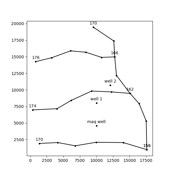
Three wells are present. Well 1 is screened in aquifer 0 and has a discharge of 1000 m\(^3\)/d, well 2 is screened in aquifer 2 and has a discharge of 5000 m\(^3\)/d, and well 3 is screened in aquifers 1 and 2 and has a total discharge of 5000 m\(^3\)/d. A constant recharge through the upper boundary of aquifer 0 is simulated by one large circular infiltration area that covers the entire model area; the recharge rate is 0.2 mm/day. A head of 175 m is specified in layer 0 at the upper righthand corner of the model domain. A layout of all analytic elements, except the boundary of the infiltration area, is shown in Figure 1.

Table 1: Aquifer data for Exercise 2

Layer	\(k\) (m/d)	\(z_b\) (m)	\(z_t\)	\(c\) (days)	\(n\) (-)	\(n_{ll}\) (-)
Aquifer 0	2	140	165	-	0.3	-
Leaky Layer 1	-	120	140	2000	-	0.2
Aquifer 1	6	80	120	-	0.25	-
Leaky Layer 2	-	60	80	20000	-	0.25
Aquifer 2	4	0	60	-	0.3	-

Figure 1: Layout of elements for Exercise 2. Heads at centers of line-sinks are indicated.

import numpy as np

import timflow.steady as tfs

figsize = (6, 6)

# Create basic model elements
ml = tfs.ModelMaq(kaq=[2, 6, 4], z=[165, 140, 120, 80, 60, 0], c=[2000, 20000], npor=0.3)
rf = tfs.Constant(ml, xr=20000, yr=20000, hr=175, layer=0)
p = tfs.CircAreaSink(ml, xc=10000, yc=10000, R=15000, N=0.0002, layer=0)
w1 = tfs.Well(ml, xw=10000, yw=8000, Qw=1000, rw=0.3, layers=0, label="well 1")
w2 = tfs.Well(ml, xw=12100, yw=10700, Qw=5000, rw=0.3, layers=2, label="well 2")
w3 = tfs.Well(ml, xw=10000, yw=4600, Qw=5000, rw=0.3, layers=[1, 2], label="maq well")
#
xy1 = [
    (833, 14261),
    (3229, 14843),
    (6094, 15885),
    (8385, 15677),
    (10781, 14895),
    (12753, 14976),
]
hls1 = [176, 166]
xy2 = [
    (356, 6976),
    (4043, 7153),
    (6176, 8400),
    (9286, 9820),
    (12266, 9686),
    (15066, 9466),
]
hls2 = [174, 162]
xy3 = [
    (1376, 1910),
    (4176, 2043),
    (6800, 1553),
    (9953, 2086),
    (14043, 2043),
    (17600, 976),
]
hls3 = [170, 156]
xy4 = [
    (9510, 19466),
    (12620, 17376),
    (12753, 14976),
    (13020, 12176),
    (15066, 9466),
    (16443, 7910),
    (17510, 5286),
    (17600, 976),
]
hls4 = [170, np.nan, 166, np.nan, 162, np.nan, np.nan, 156]

ls1 = tfs.RiverString(ml, xy=xy1, hls=hls1, layers=0)
ls2 = tfs.RiverString(ml, xy=xy2, hls=hls2, layers=0)
ls3 = tfs.RiverString(ml, xy=xy3, hls=hls3, layers=0)
ls4 = tfs.RiverString(ml, xy=xy4, hls=hls4, layers=0)

Questions:

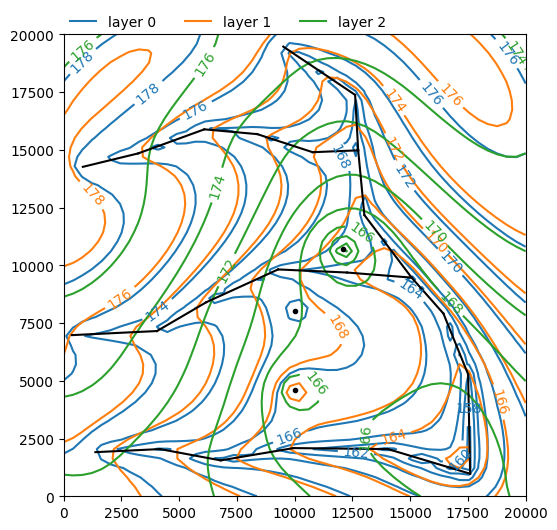
Exercise 2a

Solve the model and create a contour plot.

ml.solve()
ml.plots.contour(
    win=[0, 20000, 0, 20000],
    ngr=50,
    layers=[0, 1, 2],
    levels=10,
    color=["C0", "C1", "C2"],
    legend=True,
    figsize=figsize,
);

Number of elements, Number of equations: 9 , 25
.
.
.
.
.
.
.
.
.

solution complete

Exercise 2b

What are the heads at the three wells?

print("The head at well 1 is:", w1.headinside())
print("The head at well 2 is:", w2.headinside())
print("The head at well 3 is:", w3.headinside())

The head at well 1 is: [146.31358095]
The head at well 2 is: [138.96970957]
The head at well 3 is: [153.79826985 153.79826985]

Exercise 2c

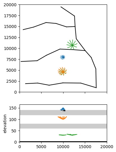
Create a contour plot including a cross-section. Create 50-year capture zones for all three wells.

axes = ml.plots.topview_and_xsection(win=[0, 20000, 0, 20000], figsize=figsize)
ml.plots.plotcapzone(
    well=w1,
    hstepmax=50,
    nt=10,
    zstart=150,
    tmax=250 * 365.25,
    orientation="both",
    ax=axes,
)
ml.plots.plotcapzone(
    well=w2, hstepmax=50, nt=10, zstart=30, tmax=250 * 365.25, orientation="both", ax=axes
)
ml.plots.plotcapzone(
    well=w3, hstepmax=50, nt=10, zstart=30, tmax=250 * 365.25, orientation="both", ax=axes
)
ml.plots.plotcapzone(
    well=w3,
    hstepmax=50,
    nt=10,
    zstart=100,
    tmax=250 * 365.25,
    orientation="both",
    ax=axes,
)

.
.
.
.
.
.
.
.
.
.
.
.
.
.
.
.
.
.
.
.
.
.
.
.
.
.
.
.
.
.
.
.
.
.
.
.
.
.
.
.

array([<Axes: >, <Axes: ylabel='elevation'>], dtype=object)

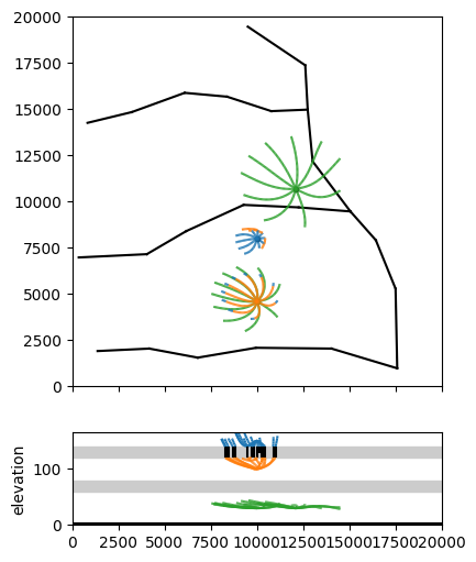
axes = ml.plots.topview_and_xsection(
    win=[0, 20000, 0, 20000], topfigfrac=0.7, figsize=figsize
)
ml.plots.plotcapzone(
    well=w1, hstepmax=50, nt=10, zstart=150, tmax=50 * 365.25, orientation="both", ax=axes
)
ml.plots.plotcapzone(
    well=w2, hstepmax=50, nt=10, zstart=30, tmax=50 * 365.25, orientation="both", ax=axes
)
ml.plots.plotcapzone(
    well=w3, hstepmax=50, nt=10, zstart=30, tmax=50 * 365.25, orientation="both", ax=axes
)
ml.plots.plotcapzone(
    well=w3, hstepmax=50, nt=10, zstart=100, tmax=50 * 365.25, orientation="both", ax=axes
)

.
.
.
.
.
.
.
.
.
.
.
.
.
.
.
.
.
.
.
.

.
.
.
.
.
.
.
.
.
.
.
.
.
.
.
.
.
.
.
.

array([<Axes: >, <Axes: ylabel='elevation'>], dtype=object)