HowTo: Model fluctuating head boundaries with timflow

This notebook shows how fluctuating head boundaries, such as a head with a varying river, can be modeled with timflow. The example is for a cross-sectional model, but the same holds for a two-dimensional model.

import matplotlib.pyplot as plt
import numpy as np

import timflow.transient as tft

Define parameters for a single unconfined aquifer. The head in the river fluctuates as a cosine with period \(\tau\).

# parameters
k = 20.0  # hydraulic conductivity, m/d
H = 50.0  # thickness of aquifer, m
T = k * H  # transmissivity, m^2/d
S = 0.1  # storage coefficient, -
tau = 0.5  # tidal period, d

The analytic solution for the head is given by the following function (see Bakker and Post, 2020).

# solution for unit amplitude
def head_river(t, tau, tp=0):
    return np.cos(2 * np.pi * (t - tp) / tau)


def analytic_head(x, t, tau, S, T, tp=0):
    B = np.exp(-x * np.sqrt(S * np.pi / (T * tau)))
    ts = x * np.sqrt(S * tau / (4 * np.pi * T))
    return B * np.cos(2 * np.pi * (t - tp - ts) / tau)

The analytic solution is for a river with varying head that has been varying for ever. In timflow.transient, head is simulated for several days to get the model to spin-up. In interpreting the results, we only look at the heads in the final tidal period.

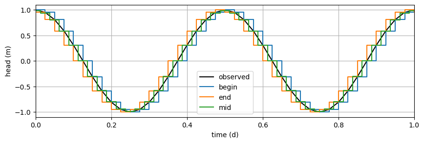
In timflow.transient, the specified head in a river is constant for a period. For example, tsandh=[(0, 1), (1, 2), (4, -2)] means the head in the river equal to 1 from \(t=0\) till \(t=1\), equal to 2 from \(t=1\) till \(t=4\) and equal to -2 thereafter. The head in a river fluctuates continuously, of course, and will be approximated by a step function.

Consider the case that the head is specified using regular time intervals \(\Delta t\) (this is not necessary of course, but practical for most applications). There are three different ways to specify a continuously vary head boundary in timflow.

• The head at time \(t\) is used for the interval from \(t\) till \(t+\Delta t\). This is referred to as begin.

• The head at time \(t+\Delta t\) is used for the interval from \(t\) till \(t+\Delta t\). This is referred to as end.

• The average between the heads at \(t\) and \(t+\Delta t\) is used for the interval from \(t\) till \(t+\Delta t\). This is referred to as mid.

A graph for these three options is shown below.

tmax = 5  # day
delt = 0.025  # day
t = np.arange(0, tmax, delt)
hexact = head_river(t, tau)
hbegin = head_river(t, tau)
hend = head_river(t + delt, tau)
hmid = 0.5 * (head_river(t - delt / 2, tau) + head_river(t + delt / 2, tau))
tmid = np.hstack((0, 0.5 * (t[:-1] + t[1:])))
# plot
plt.figure(figsize=(10, 3))
plt.plot(t, hexact, "k", label="observed")
plt.step(t, hbegin, where="post", label="begin")
plt.step(t, hend, where="post", label="end")
plt.step(tmid, hmid, where="post", label="mid")
plt.xlim(0, 1)
plt.xlabel("time (d)")
plt.ylabel("head (m)")
plt.legend()
plt.grid()

A model is created for all three options.

mlbegin = tft.ModelXsection(naq=1, tmin=1e-4, tmax=1e2)
xsection = tft.XsectionMaq(
    model=mlbegin, x1=-np.inf, x2=np.inf, kaq=k, z=[0, -H], Saq=S, phreatictop=True
)
lsriver = tft.River1D(model=mlbegin, xls=0, tsandh=list(zip(t, hbegin, strict=True)))
mlbegin.solve(silent=True)
#
mlmid = tft.ModelXsection(naq=1, tmin=1e-4, tmax=1e2)
xsection = tft.XsectionMaq(
    model=mlmid, x1=-np.inf, x2=np.inf, kaq=k, z=[0, -H], Saq=S, phreatictop=True
)
lsriver = tft.River1D(model=mlmid, xls=0, tsandh=list(zip(tmid, hmid, strict=True)))
mlmid.solve(silent=True)
#
mlend = tft.ModelXsection(naq=1, tmin=1e-4, tmax=1e2)
xsection = tft.XsectionMaq(
    model=mlend, x1=-np.inf, x2=np.inf, kaq=k, z=[0, -H], Saq=S, phreatictop=True
)
lsriver = tft.River1D(model=mlend, xls=0, tsandh=list(zip(t, hend, strict=True)))
mlend.solve(silent=True)

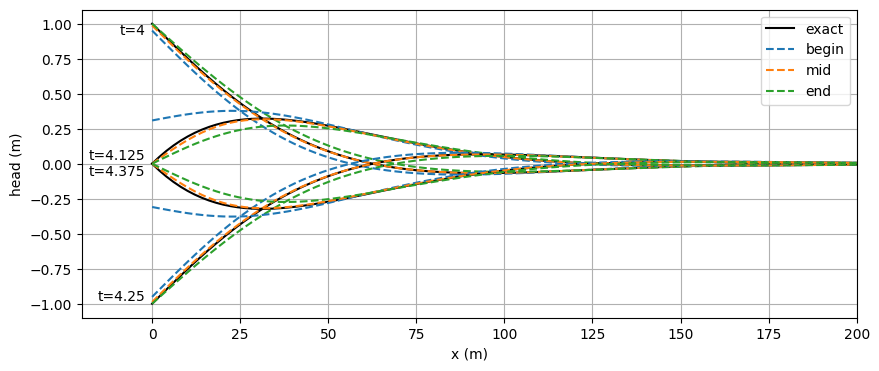
Let’s compare the output for all three options. First we look at the head along \(x\) at 4 moments in the tidal period. As we can see the mid option best matches the analytical solution. The timflow and exact solutions are closer together when the interval \(\Delta t\) is reduced.

x = np.linspace(0, 200, 100)
tlist = [4, 4.125, 4.25, 4.375]
plt.figure(figsize=(10, 4))
for tp in tlist:
    hex = analytic_head(x, tp, tau, S, T)
    plt.plot(x, hex, "k")
    for i, ml in enumerate([mlbegin, mlmid, mlend]):
        h = ml.headalongline(x, 0, tp)
        plt.plot(x, h[0, 0], "C" + str(i), linestyle="--")
plt.text(-2, 1, "t=4", ha="right", va="top")
plt.text(-2, 0.01, "t=4.125", ha="right", va="bottom")
plt.text(-2, -0.01, "t=4.375", ha="right", va="top")
plt.text(-2, -1, "t=4.25", ha="right", va="bottom")
plt.xlim(-20, 200)
plt.legend(["exact", "begin", "mid", "end"])
plt.xlabel("x (m)")
plt.ylabel("head (m)")
plt.grid()

Next we compare the head at \(x=50\) m for the last tidal period. Here we can clearly see that the begin and end result in solutions that trail and lead the analytic solution, respectively. The mid option matches nicely with the analytical solution.

plt.figure(figsize=(10, 3))
tp = np.linspace(4.5, 5, 100)
hex = analytic_head(50, tp, tau, S, T)
plt.plot(tp, hex, "k")
for ml in [mlbegin, mlmid, mlend]:
    h = ml.head(50, 0, tp)
    plt.plot(tp, h[0], "--")
plt.legend(["exact", "begin", "mid", "end"])
plt.xlabel("time (d)")
plt.ylabel("head (m)")
plt.title("head at x=50 m")
plt.grid()

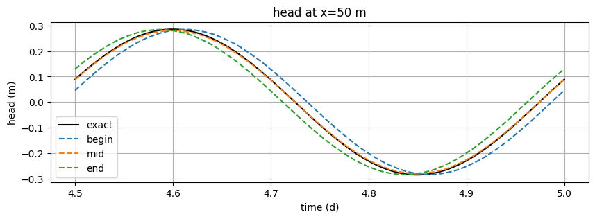
In conclusion, when modeling fluctuating boundary conditions in timflow, use the mid approximation as the input time series for your model.