Synthetic Pumping Test - Calibration

import matplotlib.pyplot as plt
import numpy as np

from timflow import transient as tft

plt.rcParams["figure.figsize"] = (6, 4)

Use observation times from Oude Korendijk

drawdown = np.loadtxt("../04pumpingtests/data/oudekorendijk_h30.dat")

tobs = drawdown[:, 0] / 60 / 24
robs = 30
Q = 788

Generate data

ml = tft.ModelMaq(kaq=60, z=(-18, -25), Saq=1e-4, tmin=1e-5, tmax=1)
w = tft.Well(ml, xw=0, yw=0, rw=0.1, tsandQ=[(0, 788)], layers=0)
ml.solve()
rnd = np.random.default_rng(2)
hobs = ml.head(robs, 0, tobs)[0] + 0.05 * rnd.random(len(tobs))

self.neq  1
solution complete

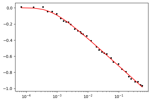
See if timflow.transient can find aquifer parameters back

cal = tft.Calibrate(ml)
cal.set_parameter(name="kaq", layers=0, initial=100)
cal.set_parameter(name="Saq", layers=0, initial=1e-3)
cal.series(name="obs1", x=robs, y=0, layer=0, t=tobs, h=hobs)
cal.fit()

.................
.................
Fit succeeded.

cal.parameters

	layers	optimal	std	perc_std	pmin	pmax	initial	inhoms	parray
kaq_0_0	0	59.871288	0.670178	1.119365	-inf	inf	100.000	None	[[59.871287575268404]]
Saq_0_0	0	0.000121	0.000004	3.633643	-inf	inf	0.001	None	[[0.00012118965722715004]]

print("rmse:", cal.rmse())

rmse: 0.014201293661013786

hm = ml.head(robs, 0, tobs, 0)
plt.semilogx(tobs, hobs, ".k")
plt.semilogx(tobs, hm[0], "r");

print("correlation matrix")
print(cal.fitresult.covar)

correlation matrix
[[ 4.49139190e-01 -2.49689096e-06]
 [-2.49689096e-06  1.93916909e-11]]

Fit with scipy.least_squares (not recommended)

cal = tft.Calibrate(ml)
cal.set_parameter(name="kaq", layers=0, initial=100)
cal.set_parameter(name="Saq", layers=0, initial=1e-3)
cal.series(name="obs1", x=robs, y=0, layer=0, t=tobs, h=hobs)
cal.fit_least_squares(report=True)

...............
....
................
.....
...
         layers    optimal       std  perc_std  pmin  pmax  initial inhoms  \
kaq_0_0       0  59.870756  0.659973  1.102330  -inf   inf  100.000   None   
Saq_0_0       0   0.000121  0.000004  3.592251  -inf   inf    0.001   None   

                             parray  
kaq_0_0      [[59.870755786046594]]  
Saq_0_0  [[0.00012119450964376704]]  
[6.59973159e-01 4.35361135e-06]
[[ 4.35564571e-01 -2.42917590e-06]
 [-2.42917590e-06  1.89539318e-11]]
[[ 1.         -0.84544047]
 [-0.84544047  1.        ]]

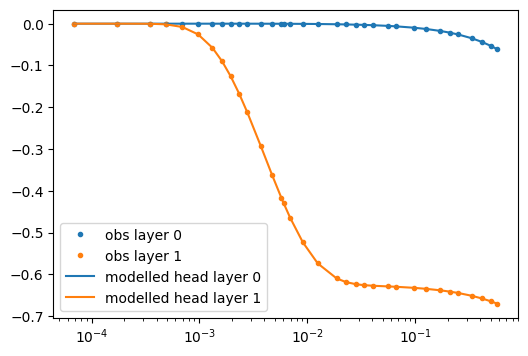
Calibrate parameters in multiple layers

Example showing how parameters can be optimized when multiple layers share the same parameter value.

ml = tft.ModelMaq(
    kaq=[10.0, 10.0],
    z=(-10, -16, -18, -25),
    c=[10.0],
    Saq=[0.1, 1e-4],
    tmin=1e-5,
    tmax=1,
)
w = tft.Well(ml, xw=0, yw=0, rw=0.1, tsandQ=[(0, 788)], layers=1)
ml.solve()
hobs0 = ml.head(robs, 0, tobs, layers=[0])[0]
hobs1 = ml.head(robs, 0, tobs, layers=[1])[0]

self.neq  1
solution complete

cal.parameters

	layers	optimal	std	perc_std	pmin	pmax	initial	inhoms	parray
kaq_0_0	0	59.870756	0.659973	1.102330	-inf	inf	100.000	None	[[59.870755786046594]]
Saq_0_0	0	0.000121	0.000004	3.592251	-inf	inf	0.001	None	[[0.00012119450964376704]]

cal = tft.Calibrate(ml)
cal.set_parameter(
    name="kaq", layers=[0, 1], initial=20.0, pmin=0.0, pmax=30.0
)  # layers 0 and 1 have the same k-value
cal.set_parameter(name="Saq", layers=0, initial=1e-3, pmin=1e-5, pmax=0.2)
cal.set_parameter(name="Saq", layers=1, initial=1e-3, pmin=1e-5, pmax=0.2)
cal.set_parameter(name="c", layers=1, initial=1.0, pmin=0.1, pmax=200.0)
cal.series(name="obs0", x=robs, y=0, layer=0, t=tobs, h=hobs0)
cal.series(name="obs1", x=robs, y=0, layer=1, t=tobs, h=hobs1)
cal.fit(report=False)
display(cal.parameters)

......
.
...
.
...
.....
.
...
.
....
....
.
...
.
....
.....
....
....
......
....
...
.......
....
....
......
...
.....
......
...
.....
.....
.
Fit succeeded.

	layers	optimal	std	perc_std	pmin	pmax	initial	inhoms	parray
kaq_0_1	[0, 1]	9.998813	3.275126e-04	0.003276	0.00000	30.0	20.000	None	[[9.998812542977381, 9.998812542977381]]
Saq_0_0	0	0.100010	1.041096e-07	0.000104	0.00001	0.2	0.001	None	[[0.10000993019005114]]
Saq_1_1	1	0.000100	1.175972e-09	0.001176	0.00001	0.2	0.001	None	[[9.999506259756452e-05]]
c_1_1	1	9.999649	9.921790e-05	0.000992	0.10000	200.0	1.000	None	[[9.999649350868319]]

plt.semilogx(tobs, hobs0, ".C0", label="obs layer 0")
plt.semilogx(tobs, hobs1, ".C1", label="obs layer 1")

hm = ml.head(robs, 0, tobs)
plt.semilogx(tobs, hm[0], "C0", label="modelled head layer 0")
plt.semilogx(tobs, hm[1], "C1", label="modelled head layer 1")

plt.legend(loc="best");

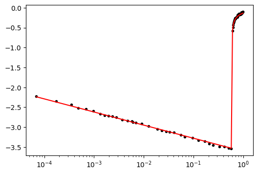
Generate data for head measured in well

tobs2 = np.hstack((tobs, np.arange(0.61, 1, 0.01)))

ml = tft.ModelMaq(kaq=60, z=(-18, -25), Saq=1e-4, tmin=1e-5, tmax=1)
w = tft.Well(ml, xw=0, yw=0, rw=0.3, res=0.02, tsandQ=[(0, 788), (0.6, 0)], layers=0)
ml.solve()
rnd = np.random.default_rng(2)
hobs2 = w.headinside(tobs2)[0] + 0.05 * rnd.random(len(tobs2))

self.neq  1
solution complete

cal = tft.Calibrate(ml)
cal.set_parameter(name="kaq", layers=0, initial=100)
cal.set_parameter(name="Saq", layers=0, initial=1e-3)
cal.set_parameter_by_reference(name="res", parameter=w.res[:], initial=0.05)
cal.seriesinwell(name="obs1", element=w, t=tobs2, h=hobs2)
cal.fit()

..............
..
.............
...
.............
...
............
....
............
....
.............
...
..............
..
...............
.
................
.
................
.
................
..
...............
.................
.................
.................
.................
.................
.................
.................
..................
.................
.................
.................
.................
....
Fit succeeded.

hm = w.headinside(tobs2)
plt.semilogx(tobs2, hobs2, ".k")
plt.semilogx(tobs2, hm[0], "r");