2. Slug Test - Falling Head

Import packages

import matplotlib.pyplot as plt
import numpy as np
import pandas as pd

import timflow.transient as tft

plt.rcParams["figure.figsize"] = [5, 3]

Introduction and Conceptual Model

This slug test, taken from the AQTESOLV examples (Duffield, 2007), was reported in Batu (1998).

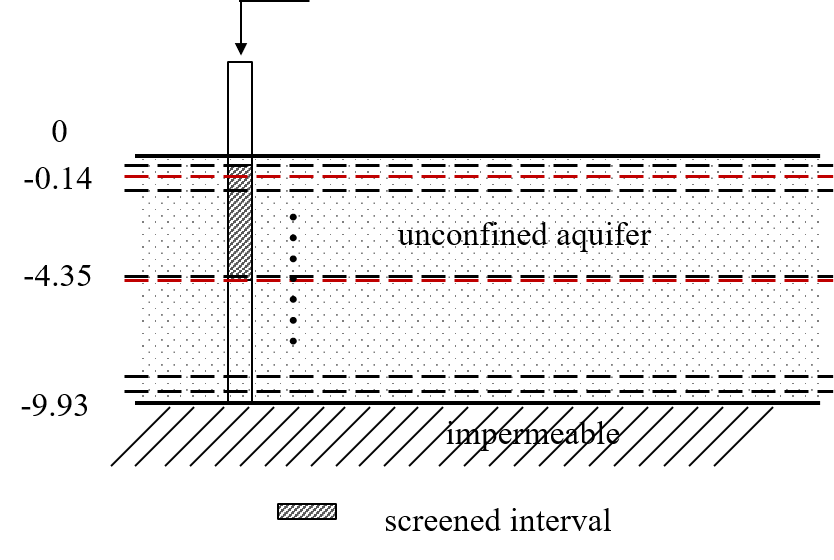
A well partially penetrates a sandy unconfined aquifer that has a saturated depth of 32.57 ft. The top of the screen is located 0.47 ft below the water table and has 13.8 ft in length. The well and casing radii are 5 and 2 inches, respectively. The slug displacement is 1.48 ft. Head change has been recorded at the slug well.

Load data

data = np.loadtxt("data/falling_head.txt", skiprows=2)
to = data[:, 0] / 60 / 60 / 24  # convert time from seconds to days
ho = (10 - data[:, 1]) * 0.3048  # convert drawdown from ft to meters

Parameters and model

rw = 5 * 0.0254  # well radius in m (5 inch = 0.127 m)
rc = 2 * 0.0254  # well casing radius in m (2 inch = 0.0508 m)
L = 13.8 * 0.3048  # screen length in m (13.8 ft = 4.2 m)
b = -32.57 * 0.3048  # aquifer thickness in m (-32.57 ft = -9.92 m)
zt = -0.47 * 0.3048  # depth to top of the screen in m (-0.47 ft = -0.14 m)
H0 = 1.48 * 0.3048  # initial displacement in the well in m (1.48 ft = 0.4511 m)
zb = zt - L  # bottom of the screen in m

convert measured displacement into volume

Q = np.pi * rc**2 * H0
print(f"slug: {Q:.5f} m^3")

slug: 0.00366 m^3

We will create a multi-layer model. For this, we divide the second and third layers into 0.5 m thick layers.

# The thickness of each layer is set to be 0.5 m
z0 = np.arange(zt, zb, -0.5)
z1 = np.arange(zb, b, -0.5)
zlay = np.append(z0, z1)
zlay = np.append(zlay, b)
zlay = np.insert(zlay, 0, 0)
nlay = len(zlay) - 1  # number of layers
Saq = 1e-4 * np.ones(nlay)
Saq[0] = 0.1

ml = tft.Model3D(
    kaq=10, z=zlay, Saq=Saq, kzoverkh=1, tmin=1e-5, tmax=0.01, phreatictop=True
)
w = tft.Well(
    ml,
    xw=0,
    yw=0,
    rw=rw,
    tsandQ=[(0, -Q)],
    layers=[1, 2, 3, 4, 5, 6, 7, 8],
    rc=rc,
    wbstype="slug",
)
ml.solve()

self.neq  8
solution complete

Estimate aquifer parameters

cal = tft.Calibrate(ml)
cal.set_parameter(name="kaq", layers=list(range(nlay)), initial=10, pmin=0)
cal.set_parameter(name="Saq", layers=list(range(nlay)), initial=1e-4, pmin=0)
cal.seriesinwell(name="obs", element=w, t=to, h=ho)
cal.fit(report=True)

.......
........
........
........
.
Fit succeeded.
[[Fit Statistics]]
    # fitting method   = leastsq
    # function evals   = 29
    # data points      = 27
    # variables        = 2
    chi-square         = 0.00108531
    reduced chi-square = 4.3413e-05
    Akaike info crit   = -269.286523
    Bayesian info crit = -266.694850
[[Variables]]
    kaq_0_21:  0.49529205 +/- 0.02255769 (4.55%) (init = 10)
    Saq_0_21:  4.0631e-04 +/- 1.0398e-04 (25.59%) (init = 0.0001)
[[Correlations]] (unreported correlations are < 0.100)
    C(kaq_0_21, Saq_0_21) = -0.9593

display(cal.parameters)
print("RMSE:", cal.rmse())

	layers	optimal	std	perc_std	pmin	pmax	initial	inhoms	parray
kaq_0_21	[0, 1, 2, 3, 4, 5, 6, 7, 8, 9, 10, 11, 12, 13,...	0.495292	0.022558	4.554423	0.0	inf	10.0000	None	[[0.49529205203295823, 0.49529205203295823, 0....
Saq_0_21	[0, 1, 2, 3, 4, 5, 6, 7, 8, 9, 10, 11, 12, 13,...	0.000406	0.000104	25.591996	0.0	inf	0.0001	None	[[0.00040631090961307237, 0.000406310909613072...

RMSE: 0.006340094887655789

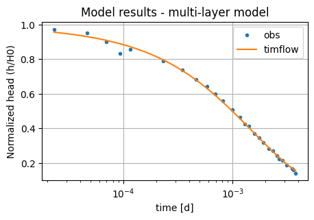
tm = np.logspace(np.log10(to[0]), np.log10(to[-1]), 100)
hm = w.headinside(tm)
plt.semilogx(to, ho / H0, ".", label="obs")
plt.semilogx(tm, hm[0] / H0, label="timflow")
plt.xlabel("time [d]")
plt.ylabel("Normalized head (h/H0)")
plt.title("Model results - multi-layer model")
plt.legend()
plt.grid()

Comparison of results

Here, we reproduce the work of Yang (2020) to check the timflow performance in analysing slug tests. We compare the solution in timflow with the KGS analytical model (Hyder et al. 1994) implemented in AQTESOLV (Duffield, 2007). AQTESOLV parameters are quite different from the set parameters in timflow. Furthermore, AQTESOLV also has a better RMSE performance.

t = pd.DataFrame(
    columns=["k [m/d]", "Ss [1/m]", "RMSE [m]"],
    index=["timflow-multi", "AQTESOLV"],
)

t.loc["timflow-multi"] = np.append(cal.parameters["optimal"].values, cal.rmse())
t.loc["AQTESOLV"] = [2.616, 7.894e-5, 0.001197]

t_formatted = t.style.format(
    {"k [m/d]": "{:.2f}", "Ss [1/m]": "{:.2e}", "RMSE [m]": "{:.3f}"}
)
t_formatted

	k [m/d]	Ss [1/m]	RMSE [m]
timflow-multi	0.50	4.06e-04	0.006
AQTESOLV	2.62	7.89e-05	0.001

References

• Batu, V. (1998), Aquifer hydraulics: a comprehensive guide to hydrogeologic data analysis, John Wiley & Sons

• Duffield, G.M. (2007), AQTESOLV for Windows Version 4.5 User’s Guide, HydroSOLVE, Inc., Reston, VA.

• Hyder, Z., Butler Jr, J.J., McElwee, C.D. and Liu, W. (1994), Slug tests in partially penetrating wells, Water Resources Research 30, 2945–2957.