Tutorial 0: Starting a model

There are two ways to start a model:

1. ModelMaq, which is model consisting of a regular sequence of aquifer - leaky layer - aquifer - leaky layer, aquifer, etc. The top of the system can be either an aquifer or a leaky layer. The head is computed in all aquifer layers only.

2. Model3D, which is a model consisting of a stack of aquifer layers. The resistance between the aquifer layers is computed as the resistance from the middle of one layer to the middle of the next layer. Vertical anisotropy can be specified. The system may be bounded on top by a leaky layer.

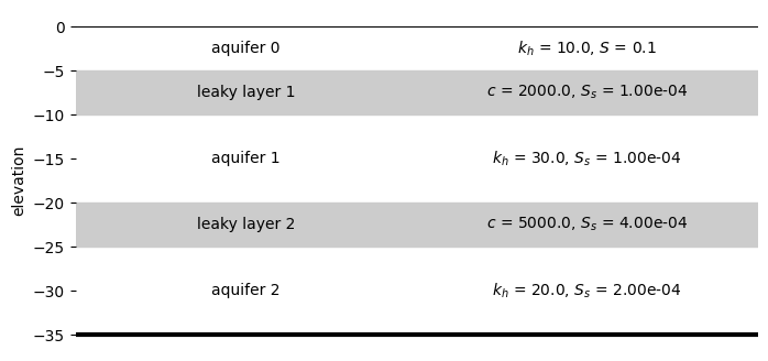
ModelMaq example

An example for ModelMaq is shown below:

• with three aquifers and two leaky layers

• top layer is phreatic (i.e. the storage coefficient is interpreted as specific yield)

• minimum time is 0.01 day, maximum time is 10 days

import timflow.transient as tft

ml = tft.ModelMaq(
    kaq=[10, 30, 20],
    z=[0, -5, -10, -20, -25, -35],
    c=[2000, 5000],
    Saq=[0.1, 1e-4, 2e-4],
    Sll=[1e-4, 4e-4],
    phreatictop=True,
    tmin=0.01,
    tmax=10,
)

ax = ml.plots.xsection(params=True)
ax.set_frame_on(False)

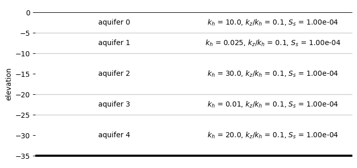
Model3D example

An example for Model3D is shown below:

• consisting of five layers all treated as aquifers, with a confined top

• with a vertical anisotropy of 0.1

• minimum time is 0.01 day, maximum time is 10 days

ml2 = tft.Model3D(
    kaq=[10, 0.025, 30, 0.01, 20],
    z=[0, -5, -10, -20, -25, -35],
    kzoverkh=0.1,
    Saq=1e-4,
    tmin=0.01,
    tmax=10,
)

ax = ml2.plots.xsection(params=True)
ax.set_frame_on(False)