Pathline tracing#
import matplotlib.pyplot as plt
import numpy as np

import timflow.transient as tft
Pathlines are computed through numerical integration of the velocity vector. Pathlines are computed with the timtrace function. The timtrace function takes as input arguments the starting locations of the pathline (xstart, ystart, zstart), a list with the starting time and end time of the pathline (tstartend), a time offset (tstartoffset), and a maximum time step (tstep). The pathline starts at the starting time plus the time offset (tstartoffset). When the starting time is at the time of a change in boundary condition (e.g., a well starts pumping), the time offset can not be smaller than tmin. The timtrace function has several keyword arguments to affect the numerical integration procedure. The hstepmax keyword is used here, which is the maximum horizontal step (in the length units consistently used throughout the model).
The timtrace function returns a dictionary with three entries:
'xyzt': 2D array with four columns: x, y, z, t along pathline'message': list with termination text messages of each section of the pathline'status': numerical indication of the result. Negative is likely undesirable.
The 'status' can be one of the following:
-2 : reached maximum number of steps before reaching maximum time
-1 : starting \(z\) value not inside aquifer
+1 : reached maximum time
+2 : reached element
The message is automatically printed to the screen unless the keyword silent is set to True.
Example 1, a pumping well in a confined aquifer#
Consider a well that starts pumping at \(t=0\) in a confined aquifer. The well is located at the origin of the coordinate system.
# parameters
Q = 100  # discharge of well, m^3/d
k = 10  # hydraulic conductivity, m/d
H = 10  # thickness of aquifer, m
Ss = 1e-4  # specific storage, m^(-1)
npor = 0.3  # porosity, -
xw = 0  # x-location of well
yw = 0  # y-location of well
rw = 0.3  # radius of well, m
tmin = 0.001  # first time of simulation after change in bc, d
ml = tft.ModelMaq(kaq=[k], z=[H, 0], Saq=[Ss], poraq=npor, tmin=tmin, tmax=1000, M=10)
w = tft.Well(ml, xw=0, yw=0, tsandQ=[(0, Q)], rw=rw)
ml.solve()
self.neq  1
solution complete
A pathline is started at \((x,y,z)=(10, 10, 0.5H)\) and time \(t=0\) and is followed for 10 days.
The output of the timtrace function is stored in the trace dictionary.
trace = tft.timtrace(
    ml,
    xstart=10,
    ystart=10,
    zstart=0.5 * H,
    tstartend=[0, 10],
    tstartoffset=tmin,
    tstep=1,
    hstepmax=2,
)
reached maximum time tmax
The entries of the trace dictionary are printed below. Note that the pathline starts at \(t=0.001\) d, which is the specified tstartoffset, that steps are taken with a length of 1 day, and that the pathline is terminated when the maximum time of 10 days is reached.
print("xyzt array of pathline:")
print(trace["xyzt"])
print("trace message:", trace["message"])
print("trace status:", trace["status"])
xyzt array of pathline:
[[1.00000000e+01 1.00000000e+01 5.00000000e+00 0.00000000e+00]
 [1.00000100e+01 1.00000100e+01 5.00000000e+00 1.00000000e-03]
 [9.78470587e+00 9.78470587e+00 5.00000000e+00 1.00100000e+00]
 [9.50979211e+00 9.50979211e+00 5.00000000e+00 2.00100000e+00]
 [9.22663761e+00 9.22663761e+00 5.00000000e+00 3.00100000e+00]
 [8.93449206e+00 8.93449206e+00 5.00000000e+00 4.00100000e+00]
 [8.63245249e+00 8.63245249e+00 5.00000000e+00 5.00100000e+00]
 [8.31944587e+00 8.31944587e+00 5.00000000e+00 6.00100000e+00]
 [7.99418666e+00 7.99418666e+00 5.00000000e+00 7.00100000e+00]
 [7.65511493e+00 7.65511493e+00 5.00000000e+00 8.00100000e+00]
 [7.30030764e+00 7.30030764e+00 5.00000000e+00 9.00100000e+00]
 [6.93723473e+00 6.93723473e+00 5.00000000e+00 1.00000000e+01]]
trace message: ['reached maximum time tmax']
trace status: [1]
When the pathline is computed for a max of 20 days (i.e., the last entry in tstartend equals 20), the well is reached before \(t=20\) d is reached
trace = tft.timtrace(
    ml,
    xstart=10,
    ystart=10,
    zstart=0.5 * H,
    tstartend=[0, 20],
    tstartoffset=tmin,
    tstep=1,
    hstepmax=2,
)
reached element of type well: Well at (0.0, 0.0)
print("last two entries in xyzt:")
print(trace["xyzt"][-2:])
last two entries in xyzt:
[[ 0.94364691  0.94364691  5.         18.8637442 ]
 [ 0.          0.          5.         19.19931262]]
When the horizontal stepsize is larger than the specified hstepmax value, the timestep is reduced. For example, specifying hstepmax=0.5 and following the pathline for 4 days gives
trace = tft.timtrace(
    ml,
    xstart=10,
    ystart=10,
    zstart=0.5 * H,
    tstartend=[0, 1],
    tstartoffset=tmin,
    tstep=1,
    hstepmax=0.1,
)
reached maximum time tmax
xyzt = trace["xyzt"]
print("xyzt:")
print(trace["xyzt"])
x0, y0, z0, t0 = xyzt[1]
x1, y1, z1, t1 = xyzt[2]
print(f"length of first step: {np.sqrt((x1 - x0) ** 2 + (y1 - y0) ** 2):.2f}")
xyzt:
[[1.00000000e+01 1.00000000e+01 5.00000000e+00 0.00000000e+00]
 [1.00000100e+01 1.00000100e+01 5.00000000e+00 1.00000000e-03]
 [9.92929932e+00 9.92929932e+00 5.00000000e+00 3.31439316e-01]
 [9.85858864e+00 9.85858864e+00 5.00000000e+00 5.95441345e-01]
 [9.78787797e+00 9.78787797e+00 5.00000000e+00 8.57431830e-01]
 [9.74925549e+00 9.74925549e+00 5.00000000e+00 1.00000000e+00]]
length of first step: 0.10
The other keyword arguments of timtrace are nstepmax=100, silent=False, and correctionstep=True. The nstepmax is the maximum number of steps. Numerical integration stops when the maximum number of steps is reached and the returned status is -2. For most practical cases, this is an undesirable result and the maximum number of steps should be increased. Setting silent=True prevents the message from being printed to the screen, which may be useful when a lot of pathlines are computed, for example in a loop. When the correctionstep is set to True (default), the numerical integration scheme is a predictor-correcter scheme. When correctionstep is set to False, the integration scheme is forward integration through time, which is less accurate but quicker.
Example 2, injection and recovery of a pumping well in a confined aquifer#
Consider a well in a confined aquifer. The well starts pumping with discharge \(Q\) at time \(t=0\) and starts injection with discharge \(Q\) at time \(t=10\) d. The well is located at the origin of the coordinate system.
ml = tft.ModelMaq(kaq=[k], z=[H, 0], Saq=[Ss], poraq=npor, tmin=tmin, tmax=1000, M=10)
w = tft.Well(ml, xw=0, yw=0, tsandQ=[(0, Q), (10, -Q)], rw=rw)
ml.solve()
self.neq  1
solution complete
A pathline is started at \((x,y,z)=(10, 10, 5)\) and followed for 20 days. The tstartend list is now [0, 10, 20]. This means that the pathline consists of two sections. The first section starts at \(t=0\) d (or really at tmin) and is followed up till \(t=10\) d. The second section starts from the endpoint at \(t=10\) d of the first section at \(t=10\) d (or really at 10+tmin days) and is followed up till \(t=20\) d. The nstepmax keyword is the maximum number of steps for each section of the pathline. There are two messages printed to the screen, one for each section.
trace = tft.timtrace(
    ml,
    xstart=10,
    ystart=10,
    zstart=0.5 * H,
    tstartend=[0, 10, 20],
    tstartoffset=tmin,
    tstep=1,
    hstepmax=2,
)
reached maximum time tmax
reached maximum time tmax
The \(x,y,z,t\) array is printed below. Note that the first section ends at \(t=10\) d. After 20 d, the pathline ends at (almost) the same location as it started. The small discrepancy is caused by numerical error of the integration scheme.
xyzt = trace["xyzt"]
print("xyzt:")
print(trace["xyzt"])
xyzt:
[[1.00000000e+01 1.00000000e+01 5.00000000e+00 0.00000000e+00]
 [1.00000100e+01 1.00000100e+01 5.00000000e+00 1.00000000e-03]
 [9.78470587e+00 9.78470587e+00 5.00000000e+00 1.00100000e+00]
 [9.50979211e+00 9.50979211e+00 5.00000000e+00 2.00100000e+00]
 [9.22663761e+00 9.22663761e+00 5.00000000e+00 3.00100000e+00]
 [8.93449206e+00 8.93449206e+00 5.00000000e+00 4.00100000e+00]
 [8.63245249e+00 8.63245249e+00 5.00000000e+00 5.00100000e+00]
 [8.31944587e+00 8.31944587e+00 5.00000000e+00 6.00100000e+00]
 [7.99418666e+00 7.99418666e+00 5.00000000e+00 7.00100000e+00]
 [7.65511493e+00 7.65511493e+00 5.00000000e+00 8.00100000e+00]
 [7.30030764e+00 7.30030764e+00 5.00000000e+00 9.00100000e+00]
 [6.93723473e+00 6.93723473e+00 5.00000000e+00 1.00000000e+01]
 [6.93724166e+00 6.93724166e+00 5.00000000e+00 1.00010000e+01]
 [7.23211139e+00 7.23211139e+00 5.00000000e+00 1.10010000e+01]
 [7.58985019e+00 7.58985019e+00 5.00000000e+00 1.20010000e+01]
 [7.93151342e+00 7.93151342e+00 5.00000000e+00 1.30010000e+01]
 [8.25906809e+00 8.25906809e+00 5.00000000e+00 1.40010000e+01]
 [8.57412453e+00 8.57412453e+00 5.00000000e+00 1.50010000e+01]
 [8.87801083e+00 8.87801083e+00 5.00000000e+00 1.60010000e+01]
 [9.17183617e+00 9.17183617e+00 5.00000000e+00 1.70010000e+01]
 [9.45653779e+00 9.45653779e+00 5.00000000e+00 1.80010000e+01]
 [9.73291597e+00 9.73291597e+00 5.00000000e+00 1.90010000e+01]
 [1.00050973e+01 1.00050973e+01 5.00000000e+00 2.00000000e+01]]
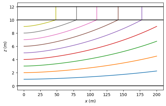
Example 3, a well in a semi-confined aquifer#
Consider an injection well in a semi-confined aquifer. The well starts injecting with discharge \(Q\) at time \(t=0\). The well is located at the origin of the coordinate system.
# parameters
k = 20  # hydraulic conductivity aquifer, m/d
H = 10  # thickness of aquifers, m
Hstar = 2  # thickness of leaky layer, m
c = 100  # resistance of leaky layer, d
Ss = 1e-4  # specific storage of both aquifers, m^(-1)
npor = 0.3  # porosity of both aquifers, -
Q = 1000  # discharge of well in aquifer 1, m^3/d
xw = 0  # x-location of well
yw = 0  # y-location of well
rw = 0.3  # radius of well, m
tmin = 0.001  # first time of simulation after change in bc, d
ml = tft.ModelMaq(
    kaq=[k],
    z=[H + Hstar, H, 0],
    c=[c],
    Saq=Ss,
    poraq=npor,
    topboundary="semi",
    tmin=tmin,
    tmax=1000,
    M=10,
)
w = tft.Well(ml, xw=0, yw=0, tsandQ=[(0, -Q)], layers=0, rw=0.3)
ml.solve()
self.neq  1
solution complete
Nine pathlines are started at the well screen at different elevations in the aquifer and followed for a max of 1000 days. Five of the nine pathlines end at the top of the semi-confining layer within the 1000 days (the five pathlines that start at the highest elevations).
plt.subplot(111, aspect=10)
zstart = np.arange(1.0, 10, 1)
for zs in zstart:
    trace = tft.timtrace(
        ml,
        xstart=rw,
        ystart=0,
        zstart=zs,
        tstartend=[0, 1000],
        tstartoffset=tmin,
        tstep=100,
        nstepmax=100,
        hstepmax=2,
        silent=True,
    )
    xyzt = trace["xyzt"]
    plt.plot(xyzt[:, 0], xyzt[:, 2])
for y in [0, H, H + Hstar]:
    plt.axhline(y, color="k")
plt.xlabel("$x$ (m)")
plt.ylabel("$z$ (m)")
Text(0, 0.5, '$z$ (m)')
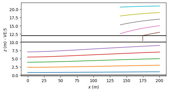
Example 4. A well in the bottom aquifer of a two-aquifer system#
Consider a pumping well in the bottom aquifer of a two-aquifer system; the aquifers are separated by a leaky layer. The well starts pumping with discharge \(Q\) at time \(t=0\). The well is located at the origin of the coordinate system.
# parameters
k0 = 20  # hydraulic conductivity aquifer 0, m/d
k1 = 40  # hydraulic conductivity aquifer 1, m/d
H = 10  # thickness of both aquifers, m
Hstar = 2  # thickness of leaky layer, m
c = 100  # resistance of leaky layer, d
Ss = 1e-4  # specific storage of both aquifers, m^(-1)
npor = 0.3  # porosity of both aquifers, -
Q = 100  # discharge of well in aquifer 1, m^3/d
xw = 0  # x-location of well
yw = 0  # y-location of well
rw = 0.3  # radius of well
ml = tft.ModelMaq(
    kaq=[k0, k1],
    z=[H + Hstar + H, H + Hstar, H, 0],
    c=[c],
    Saq=[Ss, Ss],
    poraq=npor,
    porll=npor,
    tmin=0.01,
    tmax=10000,
    M=10,
)
w = tft.Well(ml, xw=0, yw=0, tsandQ=[(0, Q)], layers=1, rw=0.3)
ml.solve()
self.neq  1
solution complete
Five pathlines are started in the top aquifer an five in the bottom aquifer at a distance of 200 m from the well and followed for a maximum of 10,000 days. The pathlines in the bottom aquifer all reach the well within that time, but the pathlines in the top aquifer don’t.
zstart = np.hstack((np.arange(1, 10, 2), np.arange(13, 22, 2)))
plt.subplot(111, aspect=5)
for zs in zstart:
    trace = tft.timtrace(
        ml,
        xstart=200,
        ystart=0,
        zstart=zs,
        tstartend=[0, 10000],
        tstartoffset=0.01,
        tstep=100,
        nstepmax=100,
        hstepmax=10,
        silent=True,
    )
    xyzt = trace["xyzt"]
    plt.plot(xyzt[:, 0], xyzt[:, 2])
for y in [0, H, H + Hstar, H + Hstar + H]:
    plt.axhline(y, color="k")
plt.xlabel("$x$ (m)")
plt.ylabel("$z$ (m) - VE:5")
Text(0, 0.5, '$z$ (m) - VE:5')
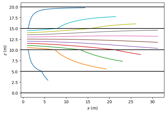
Example 5. A partially penetrating well in a four-layer system#
Consider a partially penetrating injection well. The aquifer is simulated by 4 layers and the well is screened in the second layer. The well starts pumping with discharge \(Q\) at time \(t=0\). The well is located at the origin of the coordinate system.
k = 10  # hydraulic conductivity of aquifer, m/d
H = 5  # thickness of each layer, m
Q = 100  # injection rate of well, m^3/d
Ss = 1e-4  # specific storage of both aquifers, m^(-1)
npor = 0.3  # porosity of both aquifers, -
tmin = 0.01  # minimum time, d
ml = tft.Model3D(
    kaq=k, z=np.arange(4, -1, -1) * H, Saq=Ss, poraq=npor, tmin=tmin, tmax=1000
)
w = tft.Well(ml, xw=0, yw=0, tsandQ=[(0, -Q)], layers=1, rw=0.1)
ml.solve()
self.neq  1
solution complete
Start 11 pathlines near the well and trace for 100 days.
zstart = np.linspace(10.01, 14.99, 11)
for zs in zstart:
    trace = tft.timtrace(
        ml,
        xstart=1,
        ystart=0,
        zstart=zs,
        tstartend=[0, 100],
        tstartoffset=tmin,
        tstep=5,
        nstepmax=200,
        hstepmax=2,
        silent=True,
    )
    xyzt = trace["xyzt"]
    plt.plot(xyzt[:, 0], xyzt[:, 2])
for z in np.arange(4, -1, -1) * H:
    plt.axhline(z, color="k")
plt.axis("scaled")
plt.xlabel("$x$ (m)")
plt.ylabel("$z$ (m)")
Text(0, 0.5, '$z$ (m)')