LineSink1D and LineDoublet1D

This notebook contains the examples of the LineSink1D and LineDoublet1D elements.

import matplotlib.pyplot as plt
import numpy as np
from scipy.special import erfc

import timflow.steady as tfs
import timflow.transient as tft

plt.rcParams["figure.figsize"] = (10, 4)

Define the analytical solutions for 1D confined flow in a semi-infinite field.

def ierfc(z, n):
    if n == -1:
        return 2 / np.sqrt(np.pi) * np.exp(-z * z)
    elif n == 0:
        return erfc(z)
    else:
        result = -z / n * ierfc(z, n - 1) + 1 / (2 * n) * ierfc(z, n - 2)
        return np.clip(result, a_min=0.0, a_max=None)


def bruggeman_123_02(x, t, dh, k, H, S):
    """Solution for sudden rise of the water table in a confined aquifer.

    From Bruggeman 123.02
    """
    beta = np.sqrt(S / (k * H))
    u = beta * x / (2 * np.sqrt(t))
    return dh * erfc(u)


def bruggeman_123_03(x, t, a, k, H, S):
    """Solution for linear rise of the water table in a confined aquifer.

    From Bruggeman 123.03
    """
    beta = np.sqrt(S / (k * H))
    u = beta * x / (2 * np.sqrt(t))
    return a * t * ierfc(u, 2) / ierfc(0, 2)


def bruggeman_123_05_q(x, t, b, k, H, S):
    """Solution for constant infiltration/extraction in a confined aquifer.

    From Olsthoorn, Th. 2006. Van Edelman naar Bruggeman. Stromingen 12 (2006) p5-11.
    """
    beta = np.sqrt(S / (k * H))
    u = beta * x / (2 * np.sqrt(t))
    s = 2 * b * np.sqrt(t) / np.sqrt(k * H * S) * ierfc(u, 1) / (ierfc(0, 0))
    return s

# from Analyical Groundwater Modeling, ch. 5


def h_edelman(x, t, T, S, delh, t0=0.0):
    u = np.sqrt(S * x**2 / (4 * T * (t - t0)))
    return delh * erfc(u)


def Qx_edelman(x, t, T, S, delh, t0=0.0):
    u = np.sqrt(S * x**2 / (4 * T * (t - t0)))
    return T * delh * 2 * u / (x * np.sqrt(np.pi)) * np.exp(-(u**2))

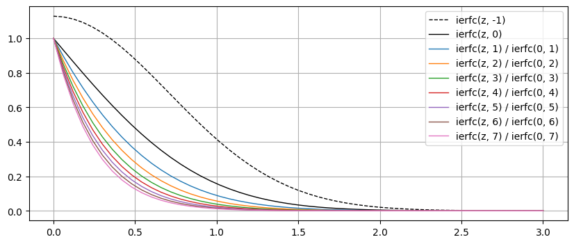
Check implementation of the iterated integral complementary error function.

Compared to figure 3 in Olsthoorn, (2006).

z = np.linspace(0, 3, 51)
ierfc_min1 = ierfc(z, -1)
ierfc0 = ierfc(z, 0)
plt.plot(z, ierfc_min1, ls="dashed", label="ierfc(z, -1)", lw=1.0, color="k")
plt.plot(z, ierfc0, ls="solid", label="ierfc(z, 0)", lw=1.0, color="k")
for n in range(1, 8):
    plt.plot(z, ierfc(z, n) / ierfc(0, n), label=f"ierfc(z, {n}) / ierfc(0, {n})", lw=1.0)
plt.legend()
plt.grid()

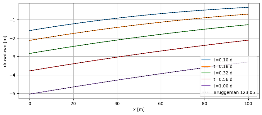
Single layer confined aquifer

Example problem confined aquifer.

k = 5
H = 10
Ss = 1e-3 / H
Q = 2.0

mlconf = tft.ModelMaq(kaq=k, z=[0, -H], Saq=Ss, tmin=1e-3, tmax=1e3, topboundary="conf")
ls = tft.DischargeLineSink1D(mlconf, tsandq=[(0, Q)], layers=[0])
mlconf.solve()

self.neq  0
No unknowns. Solution complete

Plot head along \(x\) for different times \(t\). Compare to analytical solution.

x = np.linspace(0, 100, 101)
y = np.zeros_like(x)
t = np.logspace(-1, 0, 5)

for i in range(len(t)):
    h = mlconf.headalongline(x, y, t[i])
    plt.plot(x, h.squeeze(), label=f"t={t[i]:.2f} d")
    ha = bruggeman_123_05_q(x, t[i], -Q / 2, k, H, Ss * H)  # Q/2 because 2-sided flow?
    plt.plot(x, ha, "k:")
plt.plot([], [], "k:", label="Bruggeman 123.05")
plt.legend()
plt.xlabel("x [m]")
plt.ylabel("drawdown [m]")
plt.grid()

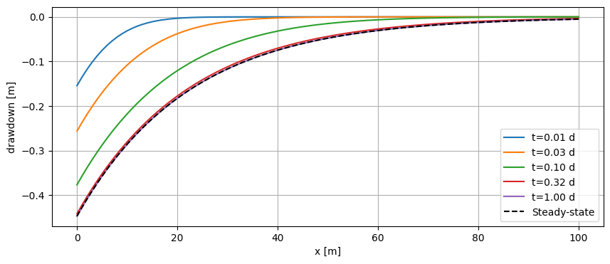
Single layer semi-confined aquifer

ml = tft.ModelMaq(kaq=k, z=[1, 0, -H], c=[10], tmin=1e-3, tmax=1e3, topboundary="semi")
ls = tft.DischargeLineSink1D(ml, tsandq=[(0, Q)], layers=[0])
ml.solve()

self.neq  0
No unknowns. Solution complete

Compare to timflow steady-state solution

mlss = tfs.ModelMaq(kaq=k, z=[1, 0, -H], c=[10], topboundary="semi", hstar=0.0)
ls = tfs.LineSink1D(mlss, 0.0, sigls=Q)
mlss.solve()

Number of elements, Number of equations: 2 , 0
No unknowns. Solution complete

Plot head along \(x\) for different times \(t\).

x = np.linspace(0, 100, 101)
y = np.zeros_like(x)
t = np.logspace(-2, 0, 5)

for i in range(len(t)):
    h = ml.headalongline(x, y, t[i])
    plt.plot(x, h.squeeze(), label=f"t={t[i]:.2f} d")

hss = mlss.headalongline(x, y)
plt.plot(x, hss.squeeze(), "k--", label="Steady-state")
plt.legend()
plt.xlabel("x [m]")
plt.ylabel("drawdown [m]")
plt.grid()

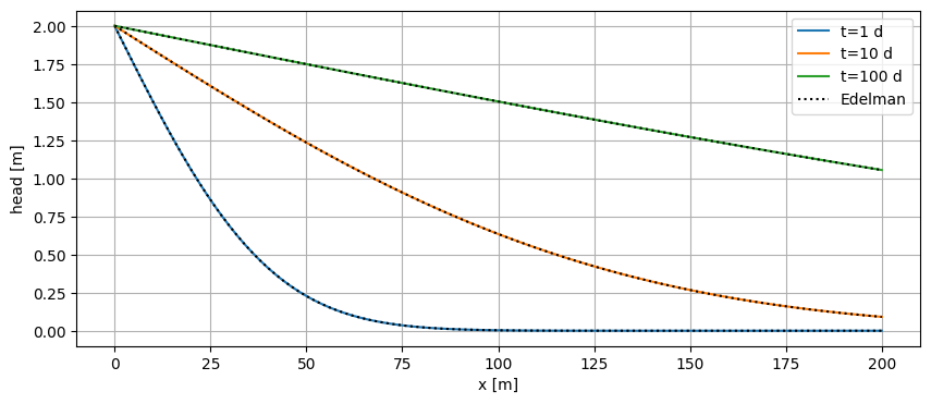
Sudden change in water level

# from Analyical Groundwater Modeling, ch. 5, p. 72
k = 10.0
H = 10.0
S = 0.2
delh = 2.0
t0 = 0.0

mlconf = tft.ModelMaq(
    kaq=k, z=[0, -H], Saq=S, tmin=1, tmax=1e2, topboundary="conf", phreatictop=True
)
hls = tft.River1D(mlconf, tsandh=[(0, delh)], layers=[0])
mlconf.solve()

self.neq  1
solution complete

Compute head along \(x\) for t = 1, 10 and 100 days. Compare to analytical solution.

x = np.linspace(0, 200, 101)
y = np.zeros_like(x)
t = np.logspace(0, 2, 3)

for i in range(len(t)):
    h = mlconf.headalongline(x, y, t[i])
    plt.plot(x, h.squeeze(), label=f"t={t[i]:.0f} d")
    ha = h_edelman(x, t[i], k * H, S, delh, t0)
    plt.plot(x, ha, "k:")

plt.plot([], [], c="k", ls="dotted", label="Edelman")
plt.legend()
plt.xlabel("x [m]")
plt.ylabel("head [m]")
plt.grid()

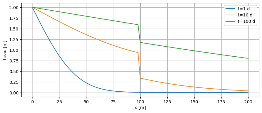
Leaky Wall

Use the previous problem but add a leaky wall at x=100 m with resistance 10 days.

# from Analyical Groundwater Modeling, ch. 5, p. 72
k = 10.0
H = 10.0
S = 0.2
delh = 2.0
t0 = 0.0

# add leaky wall with resistance
res = 10.0

mlconf = tft.ModelMaq(
    kaq=k, z=[0, -H], Saq=S, tmin=1, tmax=1e2, topboundary="conf", phreatictop=True
)
hls = tft.River1D(mlconf, xls=0.0, tsandh=[(0, delh)], layers=[0])
ld = tft.LeakyWall1D(mlconf, xld=100.0, res=res, layers=[0])
mlconf.solve()

self.neq  2
solution complete

x = np.linspace(0, 200, 101)
y = np.zeros_like(x)
t = np.logspace(0, 2, 3)

for i in range(len(t)):
    h = mlconf.headalongline(x, y, t[i])
    plt.plot(x, h.squeeze(), label=f"t={t[i]:.0f} d")

plt.legend()
plt.xlabel("x [m]")
plt.ylabel("head [m]")
plt.grid()

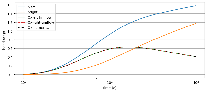
Check boundary condition along wall

dx = 1e-6
t = np.logspace(0, 2, 100)
hleft = mlconf.head(100 - dx, 0, t)
hright = mlconf.head(100 + dx, 0, t)
disxleft, _ = mlconf.disvec(100 - dx, 0, t)
disxright, _ = mlconf.disvec(100 + dx, 0, t)
disxnum = mlconf.aq.Haq * (hleft - hright) / res
plt.semilogx(t, hleft[0], label="hleft")
plt.semilogx(t, hright[0], label="hright")
plt.semilogx(t, disxleft[0], label="Qxleft timflow")
plt.semilogx(t, disxright[0], "--", label="Qxright timflow")
plt.semilogx(t, disxnum[0], "k:", label="Qx numerical")
plt.xlabel("time (d)")
plt.ylabel("head or Qx")
plt.legend()
plt.grid()

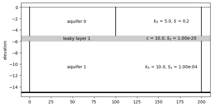
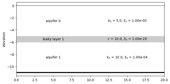
Multi-layer system

z = [0.0, -5.0, -6.0, -15.0]
Saq = [0.2, 1e-4]
c = [10.0]
k = [5.0, 10.0]
delh = 1.0
res = 10.0

mlconf = tft.ModelMaq(
    kaq=k, z=z, Saq=Saq, c=c, tmin=1, tmax=1e2, topboundary="conf", phreatictop=True
)
hls_left = tft.River1D(mlconf, xls=0.0, tsandh=[(0, delh)], layers=[0, 1])
hls_right = tft.River1D(mlconf, xls=200.0, tsandh=[(0, 0.0)], layers=[0, 1])
ld = tft.LeakyWall1D(mlconf, xld=100.0, res=res, layers=[0])
mlconf.solve()

self.neq  5
solution complete

ax = mlconf.plots.xsection([(-10, 0), (210, 0)], params=True)
for e in mlconf.elementlist:
    e.plot(ax=ax)
ax.set_xlim(-10, 210);

x = np.linspace(0, 200, 101)
y = np.zeros_like(x)
t = np.logspace(0, 2, 3)

fig, (ax0, ax1) = plt.subplots(2, 1, sharex=True, sharey=True, figsize=(10, 5))

for i in range(len(t)):
    h = mlconf.headalongline(x, y, t[i])
    ax0.plot(x, h[0].squeeze(), label=f"t={t[i]:.0f} d")
    ax1.plot(x, h[1].squeeze(), label=f"t={t[i]:.0f} d", ls="dashed")

ax0.legend(loc=(0, 1), frameon=False, ncol=3)
ax0.set_title("Layer 0")
ax1.set_xlabel("x [m]")
ax1.set_title("Layer 1")
for iax in [ax0, ax1]:
    iax.set_ylabel("head [m]")
    iax.grid()

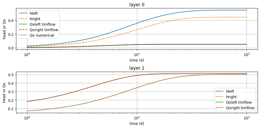
dx = 1e-6
t = np.logspace(0, 2, 100)
hleft = mlconf.head(100 - dx, 0, t)
hright = mlconf.head(100 + dx, 0, t)
disxleft, _ = mlconf.disvec(100 - dx, 0, t)
disxright, _ = mlconf.disvec(100 + dx, 0, t)
disxnum = mlconf.aq.Haq[:, np.newaxis] * (hleft - hright) / res
plt.figure(figsize=(10, 5))
for i in range(2):
    plt.subplot(2, 1, i + 1)
    plt.semilogx(t, hleft[i], label="hleft")
    plt.semilogx(t, hright[i], "--", label="hright")
    plt.semilogx(t, disxleft[i], label="Qxleft timflow")
    plt.semilogx(t, disxright[i], "--", label="Qxright timflow")
    if i == 0:  # otherwise no leaky wall
        plt.semilogx(t, disxnum[i], "k:", label="Qx numerical")
    plt.xlabel("time (d)")
    plt.ylabel("head or Qx")
    plt.title(f"layer {i}")
    plt.legend()
    plt.grid()
plt.tight_layout()

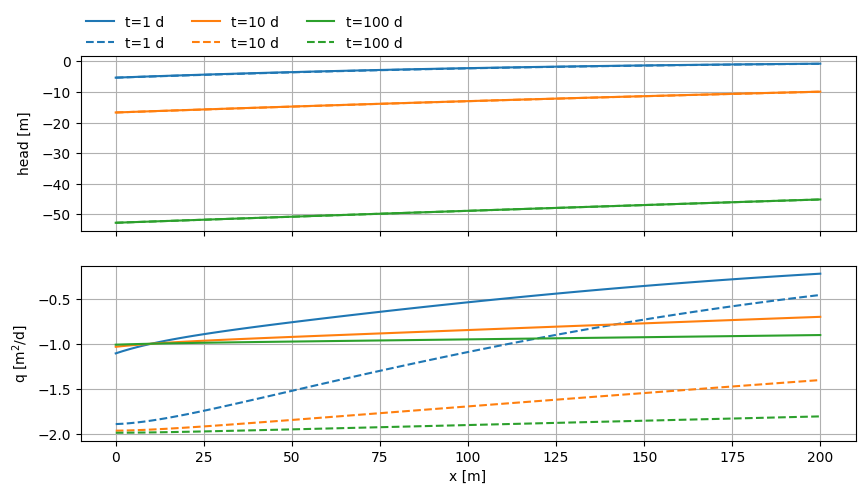
Multiscreen Linesink1D

Linesink pumping from multiple layers simultaneously with specified total discharge.

z = [0.0, -5.0, -6.0, -11.0]
Saq = [1e-3, 1e-4]
c = [10.0]
k = [5.0, 10.0]
qls = 6.0

ml = tft.ModelMaq(
    kaq=k,
    z=z,
    Saq=Saq,
    c=c,
    tmin=1,
    tmax=1e2,
    topboundary="conf",
)

ls = tft.LineSink1D(ml, xls=0.0, tsandq=[(0.0, qls)], layers=[0, 1])
ml.solve()

self.neq  2
solution complete

ax = ml.plots.xsection(xy=[(-10, 0), (10, 0)], params=True)
ml.elementlist[0].plot(ax=ax)

x = np.linspace(0, 200, 101)
y = np.zeros_like(x)
t = np.logspace(0, 2, 3)

h = ml.headalongline(x, y, t)
qx, _ = ml.disvecalongline(x, y, t)

fig, (ax0, ax1) = plt.subplots(2, 1, sharex=True, figsize=(10, 5))

for i in range(len(t)):
    (p0,) = ax0.plot(x, h[0, i].squeeze(), label=f"t={t[i]:.0f} d")
    ax0.plot(x, h[1, i].squeeze(), label=f"t={t[i]:.0f} d", ls="dashed", c=p0.get_color())
    (p1,) = ax1.plot(x, qx[0, i].squeeze(), label=f"t={t[i]:.0f} d")
    ax1.plot(
        x, qx[1, i].squeeze(), label=f"t={t[i]:.0f} d", ls="dashed", c=p1.get_color()
    )

ax0.legend(loc=(0, 1), frameon=False, ncol=3)
ax0.set_ylabel("head [m]")
ax1.set_xlabel("x [m]")
ax1.set_ylabel("q [m$^2$/d]")
for iax in [ax0, ax1]:
    iax.grid()
fig.align_ylabels()