Well in multi-layer system

import matplotlib.pyplot as plt
import numpy as np

import timflow.transient as tft

plt.rcParams["font.size"] = 8.0

Consider a three-aquifer system. Aquifer properties are given in Table 1. All aquifers have elastic storage. A well is located at \((x,y)=(0,0)\) and is screened in layer 1. The well starts pumping at time \(t=0\) with a discharge \(Q=1000\) m\(^3\)/d. The radius of the well is 0.2 m.

Table 1 - Aquifer properties for exercise 1

Layer	\(k\) (m/d)	\(c\) (d)	\(S_s\) (m\(^{-1}\))	\(z_t\) (m)	\(z_b\) (m)
Aquifer 0	1	-	0.0001	25	20
Leaky layer 1	-	1000	0	20	18
Aquifer 1	20	-	0.0001	18	10
Leaky layer 2	-	2000	0	10	8
Aquifer 2	2	-	0.0001	8	0

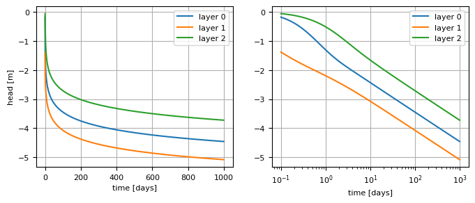
Exercise 1a

Compute the head as a function of time at \((x,y)=(50,0)\). Make a plot of the head vs. time from \(t=0.1\) till \(t=1000\) days using a linear scaling on both axis. Do the same using a logarithmic time axis.

ml = tft.ModelMaq(
    kaq=[1, 20, 2],
    z=[25, 20, 18, 10, 8, 0],
    c=[1000, 2000],
    Saq=[1e-4, 1e-4, 1e-4],
    Sll=[0, 0],
    phreatictop=False,
    tmin=0.1,
    tmax=1000,
)
w = tft.Well(ml, xw=0, yw=0, rw=0.2, tsandQ=[(0, 1000)], layers=1)
ml.solve()

t = np.logspace(-1, 3, 100)
h = ml.head(50, 0, t)
plt.figure(figsize=(8, 3))
plt.subplot(121)
plt.plot(t, h[0], label="layer 0")
plt.plot(t, h[1], label="layer 1")
plt.plot(t, h[2], label="layer 2")
plt.legend(loc="best")
plt.ylabel("head [m]")
plt.xlabel("time [days]")
plt.grid()
plt.subplot(122)
plt.semilogx(t, h[0], label="layer 0")
plt.semilogx(t, h[1], label="layer 1")
plt.semilogx(t, h[2], label="layer 2")
plt.legend(loc="best")
plt.xlabel("time [days]")
plt.grid()

self.neq  1
solution complete

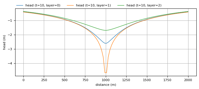
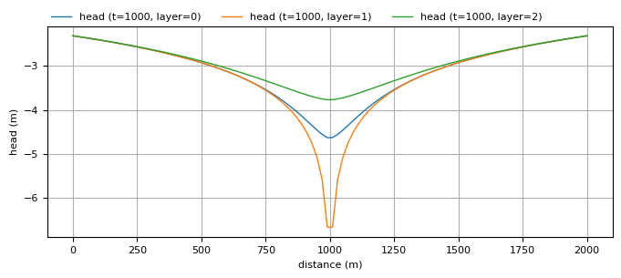
Exercise 1b

Create a plot of the head vs. distance from the well after 10 days of pumping. Plot the head in all three layers up to a distance of 1000 m from the well. Make the same plot after 1000 days of pumping. Is there much difference between 100 and 1000 days of pumping?

ml.plots.head_along_line(
    x1=-1000, x2=1000, y1=0, y2=0, npoints=100, t=10, layers=[0, 1, 2], figsize=(8, 3)
)
plt.xlabel("distance (m)")
plt.ylabel("head (m)")

ml.plots.head_along_line(
    x1=-1000, x2=1000, y1=0, y2=0, npoints=100, t=1000, layers=[0, 1, 2], figsize=(8, 3)
)
plt.xlabel("distance (m)")
plt.ylabel("head (m)")

Text(0, 0.5, 'head (m)')

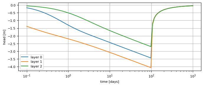
Exercise 1c

The well is turned off after 100 days. Compute the head as a function of time at \((x,y)=(50,0)\). Make a plot of the head vs. time from \(t=0.1\) till \(t=1000\) days using a logarithmic time axis.

ml = tft.ModelMaq(
    kaq=[1, 20, 2],
    z=[25, 20, 18, 10, 8, 0],
    c=[1000, 2000],
    Saq=[1e-4, 1e-4, 1e-4],
    Sll=[0, 0],
    phreatictop=False,
    tmin=0.1,
    tmax=1000,
)
w = tft.Well(ml, xw=0, yw=0, rw=0.2, tsandQ=[(0, 1000), (100, 0)], layers=1)
ml.solve()
t = np.logspace(-1, 3, 100)
h = ml.head(50, 0, t)
plt.figure(figsize=(8, 3))
plt.semilogx(t, h[0], label="layer 0")
plt.semilogx(t, h[1], label="layer 1")
plt.semilogx(t, h[2], label="layer 2")
plt.legend(loc="best")
plt.ylabel("head [m]")
plt.xlabel("time [days]")
plt.grid()

self.neq  1
solution complete

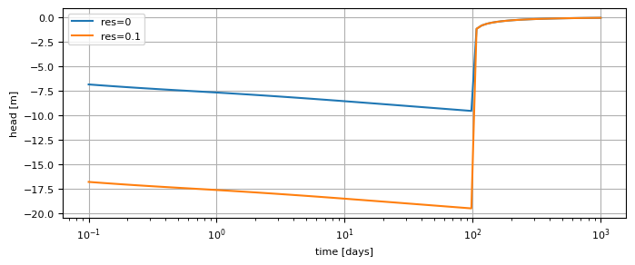
Exercise 1d

Compute the head inside the well as a function of time from \(t=0.1\) till \(t=1000\) days using a logarithmic time axis. On the same graph, plot the head inside the well vs. time when the entry resistance of the well is 0.1 days.

plt.figure(figsize=(8, 3))
h = w.headinside(t)
plt.semilogx(t, h[0], label="res=0")  # head from previous solution
w.res = 0.1
ml.solve()
h = w.headinside(t)
plt.semilogx(t, h[0], label="res=0.1")
plt.legend(loc="best")
plt.ylabel("head [m]")
plt.xlabel("time [days]")
plt.grid()

self.neq  1
solution complete

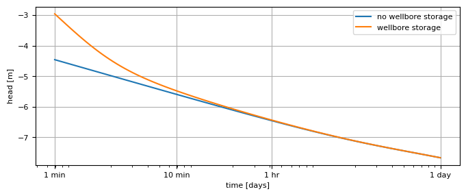
Exercise 1e

Conside again the case of a well without skin effect. Compute the head inside the well as a function of time from \(t=1\) min till \(t=1\) day using a logarithmic time axis. On the same graph, plot the head inside the well vs. time when the wellbore storage is taken into account.

tmin = 1.0 / 24 / 60  # 1 minute
ml = tft.ModelMaq(
    kaq=[1, 20, 2],
    z=[25, 20, 18, 10, 8, 0],
    c=[1000, 2000],
    Saq=[1e-4, 1e-4, 1e-4],
    Sll=[0, 0],
    phreatictop=False,
    tmin=1e-4,
    tmax=1,
)
w = tft.Well(ml, xw=0, yw=0, rw=0.2, tsandQ=[(0, 1000)], layers=1)
ml.solve()
t = np.logspace(np.log10(tmin), 0, 100)
h = w.headinside(t)
plt.figure(figsize=(8, 3))
plt.semilogx(t, h[0], label="no wellbore storage")  # head from previous solution
w.rc = 0.2
ml.solve()
h = w.headinside(t)
plt.semilogx(t, h[0], label="wellbore storage")
plt.legend(loc="best")
plt.ylabel("head [m]")
plt.xlabel("time [days]")
plt.xticks([tmin, 10 * tmin, 60 * tmin, 1], ["1 min", "10 min", "1 hr", "1 day"])
plt.grid()

self.neq  1
solution complete
self.neq  1
solution complete