1. Leaky Aquifer Test - Dalem

Import packages

import matplotlib.pyplot as plt
import numpy as np
import pandas as pd

import timflow.transient as tft

plt.rcParams["figure.figsize"] = [5, 3]

Introduction and Conceptual Model

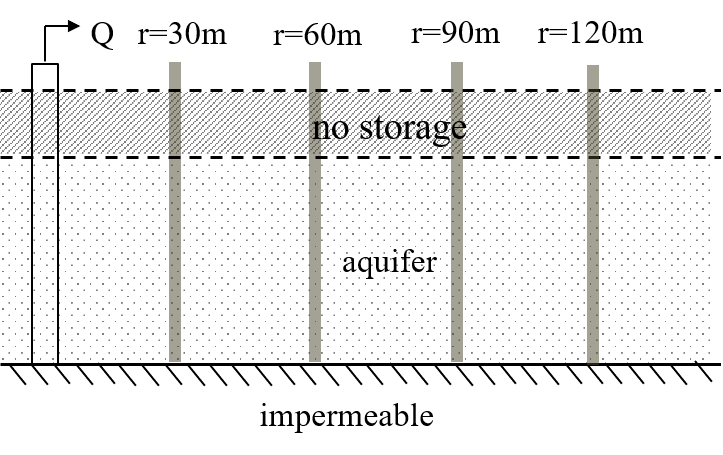
This example is a pumping test from Dalem (Kruseman et al., 1970), the Netherlands. The hydrogeological cross-section is composed of the following elements:

• an initial 8 m deep aquitard layer,

• followed by an aquifer from 8 m to 45 m depth,

• the layer underlying the aquifer is considered an aquiclude.

The pumping well is placed at the aquifer, and drawdown is recorded at four different piezometers, 30, 60, 90 and 120 m away from the well. The pumping lasted 8 hours in total at a rate of 761 m\(^3\)/d. There is a river 1500 m away from the well. The tide affects both river and well levels. Data has been previously corrected for the tide effect.

Load Data

# data of observation well 30 m away from pumping well
data1 = np.loadtxt("data/dalem_p30.txt", skiprows=1)
t1 = data1[:, 0]  # days
h1 = data1[:, 1]  # m

# data of observation well 60 m away from pumping well
data2 = np.loadtxt("data/dalem_p60.txt", skiprows=1)
t2 = data2[:, 0]
h2 = data2[:, 1]

# data of observation well 90 m away from pumping well
data3 = np.loadtxt("data/dalem_p90.txt", skiprows=1)
t3 = data3[:, 0]
h3 = data3[:, 1]

# data of observation well 120 m away from pumping well
data4 = np.loadtxt("data/dalem_p120.txt", skiprows=1)
t4 = data4[:, 0]
h4 = data4[:, 1]

Parameters and model

H = 37  # aquifer thickness in m
zt = -8  # top boundary of aquifer in m
zb = zt - H  # bottom boundary of the aquifer in m
Q = 761  # constant pumping rate in m^3/d
t = 8 / 24  # total pumping time in days (8 hours = 0.34 days)

r1 = 30  # distance from pumping well to observation well 1 in m
r2 = 60  # distance from pumping well to observation well 2 in m
r3 = 90  # distance from pumping well to observation well 3 in m
r4 = 120  # distance from pumping well to observation well 4 in m

In many situations, we cannot ignore the leakage potential of overlying and underlying formations to aquifers, and we cannot conceptualize them as confined. timflow is capable of modelling and adjusting parameters to leaky, semi-confined aquifers.

# unknown parameters: kaq, Saq, c
ml = tft.ModelMaq(
    kaq=10, z=[0, zt, zb], c=500, Saq=0.001, topboundary="semi", tmin=0.01, tmax=1
)
w = tft.Well(ml, xw=0, yw=0, tsandQ=[(0, Q), (0.34, 0)])
ml.solve(silent="True")

Estimate aquifer parameters

cal = tft.Calibrate(ml)
cal.set_parameter(name="kaq", initial=10, layers=0)
cal.set_parameter(name="Saq", initial=1e-4, layers=0)
cal.set_parameter(name="c", initial=500, pmin=0, layers=0)

cal.series(name="obs1", x=30, y=0, t=t1, h=h1, layer=0)
cal.series(name="obs2", x=60, y=0, t=t2, h=h2, layer=0)
cal.series(name="obs3", x=90, y=0, t=t3, h=h3, layer=0)
cal.series(name="obs4", x=120, y=0, t=t4, h=h4, layer=0)
cal.fit(report=True)

..................................
.........
Fit succeeded.
[[Fit Statistics]]
    # fitting method   = leastsq
    # function evals   = 40
    # data points      = 51
    # variables        = 3
    chi-square         = 0.00178546
    reduced chi-square = 3.7197e-05
    Akaike info crit   = -517.255139
    Bayesian info crit = -511.459662
[[Variables]]
    kaq_0_0:  45.3319658 +/- 1.18523874 (2.61%) (init = 10)
    Saq_0_0:  4.7623e-05 +/- 3.1043e-06 (6.52%) (init = 0.0001)
    c_0_0:    331.172052 +/- 76.1905269 (23.01%) (init = 500)
[[Correlations]] (unreported correlations are < 0.100)
    C(kaq_0_0, Saq_0_0) = -0.7707
    C(kaq_0_0, c_0_0)   = +0.7616
    C(Saq_0_0, c_0_0)   = -0.2992

display(cal.parameters)
print("RMSE:", cal.rmse())

	layers	optimal	std	perc_std	pmin	pmax	initial	inhoms	parray
kaq_0_0	0	45.331966	1.185239	2.614576	-inf	inf	10.0000	None	[[45.33196584030614]]
Saq_0_0	0	0.000048	0.000003	6.518616	-inf	inf	0.0001	None	[[4.762252808671633e-05]]
c_0_0	0	331.172052	76.190527	23.006328	0.0	inf	500.0000	None	[[331.1720519742353]]

RMSE: 0.005916842465653116

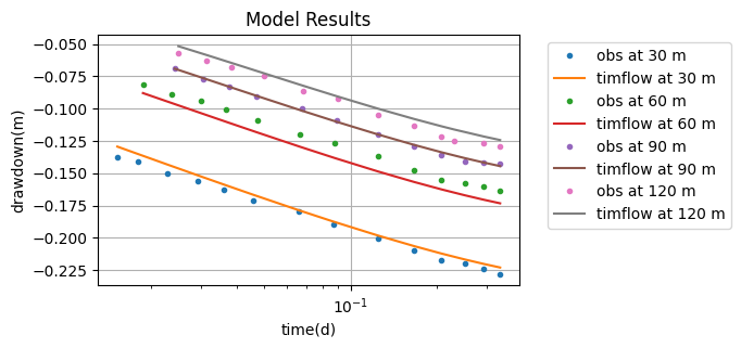
hm_1 = ml.head(r1, 0, t1)
plt.semilogx(t1, h1, ".", label="obs at 30 m")
plt.semilogx(t1, hm_1[0], label="timflow at 30 m")

hm_2 = ml.head(r2, 0, t2)
plt.semilogx(t2, h2, ".", label="obs at 60 m")
plt.semilogx(t2, hm_2[0], label="timflow at 60 m")

hm_3 = ml.head(r3, 0, t3)
plt.semilogx(t3, h3, ".", label="obs at 90 m")
plt.semilogx(t3, hm_3[0], label="timflow at 90 m")

hm_4 = ml.head(r4, 0, t4)
plt.semilogx(t4, h4, ".", label="obs at 120 m")
plt.semilogx(t4, hm_4[0], label="timflow at 120 m")

plt.xlabel("time(d)")
plt.ylabel("drawdown(m)")
plt.title("Model Results")
plt.legend(bbox_to_anchor=(1.05, 1))
plt.grid();

Comparison of results

The performance of timflow was evaluated by comparison with other numerical models and with parameter values reported in Kruseman and de Ridder (1970). The published values were obtained by graphical matching to the Hantush family of type curves (Hantush, 1955). In addition to the timflow results and the literature values, results from AQTESOLV (Duffield, 2007) and MLU (Carlson & Randall, 2012), as reported by Yang (2020), are included for comparison.

Overall, all models yield similar estimates of the aquifer hydraulic conductivity. However, the timflow results differ substantially from the MLU and AQTESOLV solutions with respect to aquitard storage and hydraulic resistance.

t = pd.DataFrame(
    columns=["k [m/d]", "Ss [1/m]", "c [d]", "RMSE [m]"],
    index=["timflow", "AQTESOLV", "MLU", "Hantush"],
)

t.loc["timflow"] = np.append(cal.parameters["optimal"].values, cal.rmse())
t.loc["AQTESOLV"] = [49.286, 4.559e-05, 745.156, 0.007245]
t.loc["MLU"] = [45.186, 3.941e-05, 769.200, 0.005941]
t.loc["Hantush"] = [45.332, 4.762e-5, 331.141, 0.005917]

t_formatted = t.style.format(
    {"k [m/d]": "{:.2f}", "Ss [1/m]": "{:.2e}", "c [d]": "{:.0f}", "RMSE [m]": "{:.2f}"}
)
t_formatted

	k [m/d]	Ss [1/m]	c [d]	RMSE [m]
timflow	45.33	4.76e-05	331	0.01
AQTESOLV	49.29	4.56e-05	745	0.01
MLU	45.19	3.94e-05	769	0.01
Hantush	45.33	4.76e-05	331	0.01

References

• Bakker, M. (2013), Semi-analytic modeling of transient multi-layer flow with TTim, Hydrogeol J 21, 935–943, https://doi.org/10.1007/s10040-013-0975-2

• Carlson, F. and Randall, J. (2012), MLU: a Windows application for the analysis of aquifer tests and the design of well fields in layered systems, Ground Water 50(4):504–510.

• Duffield, G.M., (2007), AQTESOLV for Windows Version 4.5 User’s Guide, HydroSOLVE, Inc., Reston, VA.

• Kruseman, G.P., De Ridder, N.A. and Verweij, J.M., (1970), Analysis and evaluationof pumping test data, volume 11, International institute for land reclamation and improvement The Netherlands.

• Newville, M., Stensitzki, T., Allen, D.B. and Ingargiola, A. (2014), LMFIT: Non Linear Least-Squares Minimization and Curve Fitting for Python, https://dx.doi.org/10.5281/zenodo.11813, https://lmfit.github.io/lmfit-py/intro.html (last access: August,2021).